Long term trends of pan evaporation and an analysis of its causes in Finland

(1)

causes in Finland

Toshitsugu Moroizumi†_{, Naoya Ito}††_{, Jari Koskiaho}†††_{and Sirkka Tattari}†††

† _{Graduate School of Environmental and Life Science, Okayama University, Japan}

[email protected], [email protected]

† _{Master course student at Graduate School of Environmental and Life Science}

Okayama University, 3-1-1, Tsushima-naka, Okayama, 700-8530, Japan [email protected],ac,jp

††† _{Freshwater Centre, Finnish Environment Institute, Finland}

[email protected]

††† _{Freshwater Centre, Finnish Environment Institute, Finland}

[email protected]

Abstract:

Long - term trend of pan evaporation which was a key factor of hydrologic cycle and water resources management was investigated with the long-term variation of meteorological data: precipitation, air temperature, relative humidity, and wind speed. The causes of trends of pan evaporation were revealed from two points of view: complementary relationship and Penman's equation. The variations of pan evaporation showed the decreasing trends at the 5 stations and the increasing ones in the other 2 stations. The mechanistic causes for the decreasing trends were mainly the increases of the precipitation and the aerodynamic term in Penman's equation (1948).

1. Introduction

The recent global warming causes the climate changes such as concentrated rainfall or flood, and affects the evapotranspiration which is an important factor of hydrologic cycle and water resources management. Many of the previous studies have reported the decrease trends of pan evaporation in the area of the continental climate of the middle latitude. However, few studies in the region in a high latitude area such as Finland haven't been carried out so far.

The purpose of this study is to investigate the long term variations of pan evaporation in Finland located in a high latitude using a trend analysis. In addition, the relationship between pan evaporation and meteorological elements is discussed to clarify the causes of the long-term trend of pan evaporation.

(2)

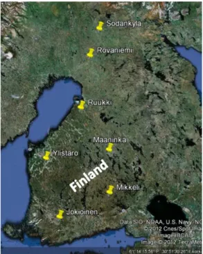
Seven meteorological stations from southern to northern parts in Finland were selected for this study (Fig. 1). Table 1 also shows those details: latitude, longitude, amplitude, and a measurement height of wind speed.

Pan evaporation data were obtained from the Finnish Environment Institute. The meteorological data : precipitation, air temperature, humidity, wind speed, and radiation (or sunshine duration), were provided by the Finnish Meteorological Institute. The pan evaporation data were measured with a Class A evaporation pan which was the most common method of measurement of open water evaporation.

The data except wind speed were the time series of daily records. The wind speed data recorded at 0600, 1200, and 1800 hours were averaged and converted the daily data.

The analysis period was 52 years (1960 - 2011). The data in June to September in each year were analyzed because there were many missing data in October to May mainly due to freezing of water. The integrated values of those 4 months in the pan evaporation and the precipitation data, and the average values of the 4 months in the other meteorological data were used.

A linear regression model which was the most commonly used method was used to detect the trend for all data. The trend slopes for the data except air temperature were showed as the percentage per decade which was normalized by the average value over the period. The trend slopes of the regression model were tested against the hypothesis of null slope by means of a one-tail t-test at a confidence level of 95 % or 99 %.

(3)

3. Results

3.1 Pan evaporation

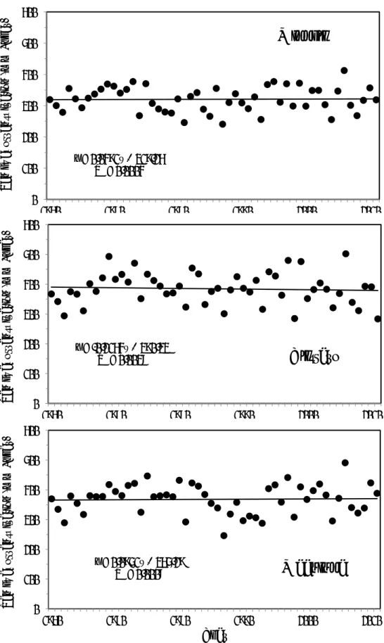
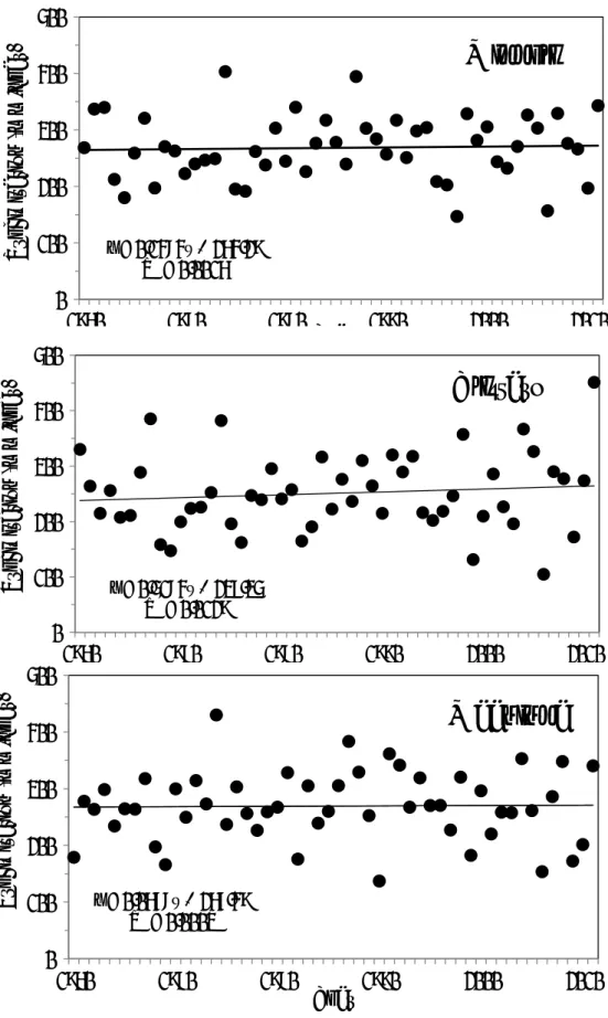
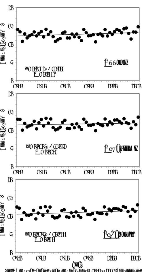
Fig. 2 shows the yearly variation of pan evaporation and its regression line. Table 2 presents the average and the trend. The pan evaporation decreased in Jokioinen, Ylistaro, Ruukki, Rovaniemi, and Sodankylä, and increased slightly in Mikkeli and Maaninka. The average decrease percentage and the average value at 7 stations were - 2.82 (%) and 343 (mm), respectively.

Station ID Name of station Latitude (N)* Longtitude (E)* Altitude (m) a.s.l Height of wind speed (m) 1201 Jokioinen 60｡_48' ₂₃｡_30' ₁₀₄ ₃₀ 2602 Mikkeli 61｡_40' ₂₇｡_13' ₁₀₁ ₁₀ 3101 Ylistaro 62｡_56' ₂₂｡_11' ₂₆ ₁₂ 3603 Maaninka 63｡_08' ₂₇｡_19' ₉₀ ₁₈ 5402 Ruukki 64｡_41' ₂₅｡_05' ₄₈ ₁₂ 7502 Rovaniemi 66｡_34' ₂₆｡_01' ₁₀₆ ₁₂ 7501 Sodankylä 67｡_22' ₂₆｡_37' ₁₇₉ ₂₂ *WGS-84 stations. y = -0.7932x + 419.8 R² = 0.0398 0 100 200 300 400 500 600 1960 1970 1980 1990 2000 2010 P an eva po tra ns pi ra ti on (m m / y ea r)

Year

Jokioinen

Fig. 2 Temporal variation of pan evaporation from 1960 to 2011. The regression line is showed together.

(4)

y = 0.0491x + 319.26 R² = 0.0004 0 100 200 300 400 500 1960 1970 1980 1990 2000 2010 P an ev apotra nsp ira ti on (m m / yea r) Year

Mikkeli

y = -0.2164x + 390.33 R² = 0.0038 0 100 200 300 400 500 600 1960 1970 1980 1990 2000 2010 Pan eva po tra ns pi ra ti on (m m / y ea r) Year

Ylistaro

y = 0.0951x + 365.29 R² = 0.0008 0 100 200 300 400 500 600 1960 1970 1980 1990 2000 2010 Pan eva po tra ns pi ra ti on (m m / y ea r) Year

Maaninka

(5)

y = -2.3625x + 392 R² = 0.4336 0 100 200 300 400 500 1960 1970 1980 1990 2000 2010 P an ev apotra nsp ira ti on (m m / yea Year

Ruukki

y = -1.8051x + 331.3 R² = 0.3693 0 100 200 300 400 500 600 1960 1970 1980 1990 2000 2010 Pa n ev apotra nsp ir atio n (mm / yea r) Year

Rovaniemi

y = -1.7269x + 361.09 R² = 0.271 0 100 200 300 400 500 600 1960 1970 1980 1990 2000 2010 Pan eva po transp ir atio n (mm / y ea r) Year

Sodankylä

(6)

3.2 Precipitation

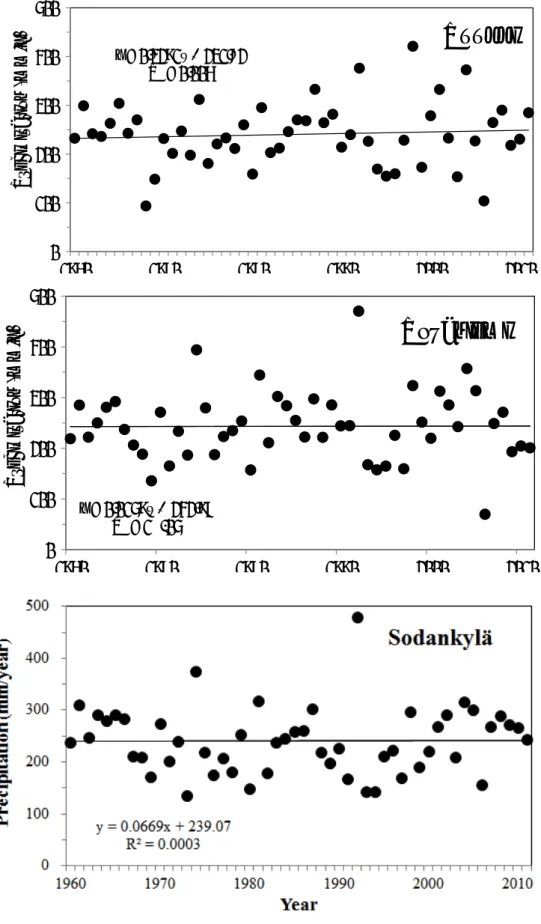
Figure 3 shows the yearly variation of precipitation and its regression line. The precipitation increased in all stations. Especially, the trends in Jokioinen, Ylistaro, and Ruukki close to sea were relatively larger than those in the other stations (Table 2). The average decrease percentage and the average value at 7 stations were 0.80 (%) and 255 (mm), respectively. y = -0.9657x + 368.44 R² = 0.1231 0 100 200 300 400 500 1960 1970 1980 1990 2000 2010 P an ev apotra nsp ira ti on (m m / yea r) Year

Average

y = 0.2757x + 265.77 R² = 0.005 0 100 200 300 400 500 1960 1970 1980 1990 2000 2010 P reci pi ta ti on (m m /y ea r) Year

Jokioinen

Fig. 3 Temporal variation of precipitation from 1960 to 2011. The regression line is showed together.

(7)

y = 0.1484x + 264.29 R² = 0.0016 0 100 200 300 400 1960 1970 1980 1990 2000 2010 P reci pi ta ti on (m m /y ea r) Year

Mikkeli

Ylistaro

Maaninka

(8)

y = 0.3291x + 231.82 R² = 0.006 0 100 200 300 400 1960 1970 1980 1990 2000 2010 P reci pi ta ti on (m m /y ) Year

Ruukki

y = 0.0159x + 242.97 R² = 1E-05 0 100 200 300 400 500 1960 1970 1980 1990 2000 2010 Pr ec ipi ta ti on (m m /y ) Year

Rovaniemi

(9)

3.3 Air temperature

Figure 4 shows the yearly variation of air temperature and its regression line. The air temperature increased in all stations (Table 2). The average decrease percentage and the average value at 7 stations were 1.65 (%) and 12.8 (℃), respectively.

y = 0.2032x + 249.82 R² = 0.0042 0 100 200 300 400 1960 1970 1980 1990 2000 2010 P reci pi ta ti on (m m /y ) Year

Average

Fig. 3 Temporal variation of precipitation from 1960 to 2011. The regression line is showed together. y = 0.0276x + 13.027 R² = 0.1578 0 5 10 15 20 1960 1970 1980 1990 2000 2010 T em pera tur e (℃ ) Year

Jokioinen

Fig. 4 Temporal variation of air temperature from 1960 to 2011. The regression line is showed together.

(10)

y = 0.0195x + 13.05 R² = 0.0861 0 5 10 15 1960 1970 1980 1990 2000 2010 T em pera tur e (℃ ) Year

Mikkeli

y = 0.0264x + 12.635 R² = 0.1557 0 5 10 15 20 1960 1970 1980 1990 2000 2010 T em pera tur e (℃ ) Year

Ylistaro

Maaninka

(11)

y = 0.0182x + 12.207 R² = 0.0774 0 5 10 15 1960 1970 1980 1990 2000 2010 T em pera tur e (℃ ) Year

Ruukki

Rovaniemi

Sodankylä

(12)

y = 0.0211x + 12.242 R² = 0.1071 0 5 10 15 1960 1970 1980 1990 2000 2010 T em peratur e (℃ ) Year

Average

(13)

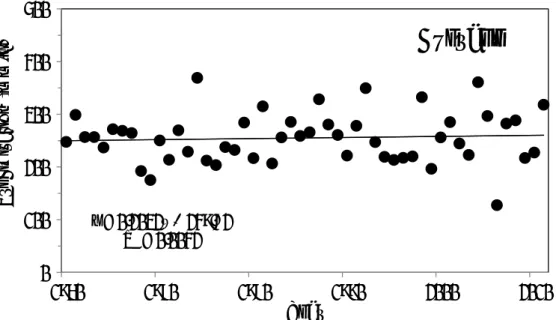
Figure 5 shows the yearly variation of relative humidity and its regression line. The relative humidity increased in the 5 stations except Mikkeli and Sodankylä (Table 2). The average decrease percentage and the average value at 7 stations were 0.90 (%) and 73.4 (%), respectively. y = -0.08x + 77.927 R² = 0.0981 60 70 80 90 100 1960 1970 1980 1990 2000 2010 Hum idi ty (% ) Year

Jokioinen

y = 0.077x + 72.376 R² = 0.1063 60 70 80 90 100 1960 1970 1980 1990 2000 2010 Hum idi ty (% ) Year

Mikkeli

Fig. 5 Temporal variation of relative humidity from 1960 to 2011. The regression line is showed together.

(14)

y = 0.1312x + 69.763 R² = 0.1566 60 70 80 90 1960 1970 1980 1990 2000 2010 Hum idi ty (% ) Year

Ylistaro

Manninka

Ruukki

(15)

y = 0.136x + 68.129 R² = 0.1547 60 70 80 90 1960 1970 1980 1990 2000 2010 Hum idi ty (% ) Year

Rovaniemi

y = -0.0304x + 73.968 R² = 0.0233 60 70 80 90 100 1960 1970 1980 1990 2000 2010 Hum idi ty (% ) Year

Sodankylä

Average

(16)

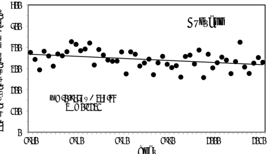
Figure 6 shows the yearly variation of wind speed and its regression line. The wind speed decreased in the 6 stations except Rovaniemi (Table 2). The average decrease percentage and the average value at 7 stations were -4.07 (%) and 2.78 (m/s), respectively. y = -0.0133x + 3.9481 R² = 0.486 0 2 4 6 1960 1970 1980 1990 2000 2010 W ind speed (m /s ) Year

Jokioinen

y = -0.0163x + 2.9413 R² = 0.5017 0 2 4 6 1960 1970 1980 1990 2000 2010 W ind speed (m /s ) Year

Mikkeli

Fig. 6 Temporal variation of wind speed from 1960 to 2011. The regression line is showed together.

(17)

y = -0.0111x + 3.1439 R² = 0.0956 0 2 4 1960 1970 1980 1990 2000 2010 W ind speed (m /s ) Year

Ylistaro

Maaninka

Ruukki

(18)

y = 0.0021x + 2.2996 R² = 0.0093 0 2 4 1960 1970 1980 1990 2000 2010 W ind speed (m /s ) Year

Rovaniemi

Sodankylä

Average

(19)

Mean Trend Mean Trend Mean Trend Mean Trend Mean Trend Mean Trend (mm y-1) (%/decade) (mm y-1) (%/decade) (℃) (℃/decade) (%) (%/decade) (%) (%/decade) (mm/d) (%/decade)

Jokioinen 399 -1.99 273 1.01 13.8 2.01 75.8 -1.06 3.60 -3.70 1.28 1.53 Mikkeli 321 0.15 268 0.55 13.6 1.44 74.4 1.03 2.51 -6.48 1.18 -6.45 Ylistaro 385 -0.56 251 2.06 13.3 1.98 73.2 1.79 2.85 -3.88 1.32 -6.79 Maaninka 368 0.26 269 0.25 13.6 1.93 72.2 1.45 2.83 -2.29 1.30 -4.52 Ruukki 329 -7.17 241 1.37 12.7 1.44 73.3 1.72 2.25 -7.36 1.10 -8.35 Rovaniemi 283 -6.37 243 0.07 11.7 0.90 71.7 1.90 2.36 0.89 1.15 -4.17 Sodankylä 315 -5.48 241 0.28 11.0 1.77 73.2 -0.42 3.08 -5.73 1.20 -2.07 Mean 343 -2.82 255 0.80 12.8 1.65 73.2 0.90 2.78 -4.07 1.22 -4.33

Wind 2nd term of penman Station

Pan evaporation Precipitation Temperature Humidity

4. Discussion

4.1 Relationship between pan evaporation and precipitation

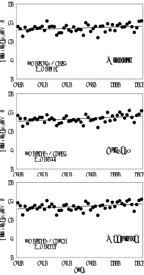
Brutsaert and Parlange (1998) discussed the cause of the decrease trend of pan evaporation using the complementary relationship (CR) of which the concept had been suggested by Bouchet (1963). The schematic diagram of the CR is shown in Figure 7. According to the CR, the pan evaporation which is a kind of potential evaporation decrease if the actual evaporation increases, vice versa. In this section, we discuss the results of this study using the CR.

The variation of precipitation showed the increase trend at all stations (Table 2). The increase of precipitation induce the increase of actual evaporation due to the increase of land moisture. Therefore, according to the CR, the increase trend of precipitation is at least one of the causes for decrease trend in the 5 stations except Mikkeli and Maaninka . Figure 8 shows the relationship between pan evaporation and precipitation. The pan evaporation decreased when the precipitation increase. However, the CR was not applicable for the results in Mikkei and Maaninka.

wind speed and the second term of Penman's equation. The bold and underline values show the 99％ significant level, and the bold ones the 95％.

low _{Soil moisture} _high

Actual evaporation Pan / Potential evaporations

Evap

orat

ion

(20)

y = -0.5101x + 538.09 R² = 0.2519 0 0.5 1 1.5 2 0 0.5 1 1.5 2 N orm al ized p na ev ap orat io n ( -) Normalized precipitaion ( - ) Jokioinen y = -0.2775x + 1.2775 R² = 0.2176 0 0.5 1 1.5 2 0 0.5 1 1.5 2 No rm al ize d pn a ev ap ora ti on ( -) Normalized precipitaion ( - ) Maaninka y = -0.3044x + 1.3044 R² = 0.3674 0 0.5 1 1.5 2 0 0.5 1 1.5 2 Norm al ized p na ev ap orat io n ( -) Normalized precipitaion ( - ) Ylistaro y = -0.5101x + 538.09 R² = 0.2519 0 0.5 1 1.5 2 0 0.5 1 1.5 2 N orm al ized p na ev ap orat io n ( -) Normalized precipitaion ( - ) Rovaniemi y = -0.3135x + 1.3135 R² = 0.2595 0 0.5 1 1.5 2 0 0.5 1 1.5 2 No rm al ize d pn a ev ap ora ti on ( -) Normalized precipitaion ( - ) Ruukki

(21)

4.2 Analysis by Penman equation

The pan evaporation has the same qualified variation as the potential evaporation, though pan evaporation tends to be larger than the potential evaporation (Brutsaert, 1982). In this section, the mechanistic cause of the trend in the pan evaporation was investigated using the potential evaporation estimated by Penman’s equation (1948) which is as follows: n ( )(₂ ) p sa a R E f u e e l γ γ γ Δ = + − Δ + Δ + (1) where EP : potential evaporation (mm･d-1)，Rn : net radiation (MJ･m-2･d-1)，u2 : wind speed at 2m height, f(u2) : wind function (m･d-1･hPa-1)［=0.26×(1+0.54u2)］，esa :

saturated water vapor pressure (hPa)，ea : water vapor pressure (hPa). The first and the

second terms on right hand in equation (1) are called a radiative and aerodynamic terms, respectively.

The normalized trends are shown in Table 2. Figure 9 shows the relationship between the normalized trends in pan evaporation and in the normalized 2nd term of equation (1). The normalized trends were decreasing at all stations, which, therefore, caused the decrease trends of pan evaporation at the 5 stations except Mikkeli and Maaninka. To investigate the mechanistic cause of the trend of the pan evaporation in more detail, we also need to analysis the right hand 1st term of Penman’s equation which is related to a radiation. y = -0.1863x + 1.1863 R² = 0.0953 0 0.5 1 1.5 2 0 0.5 1 1.5 2 N orm al ized p na ev ap orat io n ( -) Normalized precipitaion ( - ) Sodankylä y = -0.4359x + 1.4359 R² = 0.4424 0 0.5 1 1.5 2 0 0.5 1 1.5 2 N orm al ized p na ev ap orat io n ( -) Normalized precipitaion ( - ) Average

(22)

y = 0.6198x + 0.3802 R² = 0.487 0 0.5 1 1.5 2 0.00 0.50 1.00 1.50 2.00 N orm al ized p na ev ap orat io n ( -)

Normalized 2nd term of Penman ( - ) Jokioinen y = 0.3437x + 0.6563 R² = 0.2777 0 0.5 1 1.5 2 0.00 0.50 1.00 1.50 2.00 N orm al ized p na ev ap orat io n ( -)

Normalized 2nd term of Penman ( - ) Mikkeli y = 0.2958x + 0.7042 R² = 0.373 0 0.5 1 1.5 2 0.00 0.50 1.00 1.50 2.00 N orm al ized p na ev ap orat io n ( -)

Normalized 2nd term of Penman ( - ) Ylistaro y = 0.3276x + 0.6724 R² = 0.1687 0 0.5 1 1.5 2 0.00 0.50 1.00 1.50 2.00 N orm al ized p na ev ap orat io n ( -)

Normalized 2nd term of Penman ( - ) Maaninka y = 0.5636x + 0.4364 R² = 0.5872 0 0.5 1 1.5 2 0.00 0.50 1.00 1.50 2.00 N orm al ized p na ev ap orat io n ( -)

Normalized 2nd term of Penman ( - ) Ruukki y = 0.2556x + 0.7444 R² = 0.1155 0 0.5 1 1.5 2 0.00 0.50 1.00 1.50 2.00 N orm al ized p na ev ap orat io n ( -)

Normalized 2nd term of Penman ( - ) Rovaniemi

Fig. 9 Relationship between normalized 2nd term in Penman's equation and pan evaporation.

(23)

5. Conclusion

The trend analyses of pan evaporation were carried out for 7 stations in Finland located

in a high latitude. The causes of the trends of pan evaporation were revealed from two

points of view: a complementary relationship and Penman's equation. The results were follows:

(1) The variations of pan evaporation showed the decreasing trends at the 5 stations and the increasing ones in the 2 stations.

(2) The mechanistic causes for the decreasing trends in the 5 stations were mainly the increases of the precipitation and the aerodynamic term in Penman's equation.

(3) The mechanistic causes for the increasing trends in the 2 stations couldn't be revealed .

The following future works are needed:

(1) Radiation or sunshine duration is needed for estimating the right hand 1st term of Penman' s equation.

(2) The Mann-Kendall test is generally better than the T-test to asses the statistical significance of trends, though the t-test was carried out in the present study because a few studies used it.

y = 0.7003x + 0.2997 R² = 0.4222 0 0.5 1 1.5 2 0.00 0.50 1.00 1.50 2.00 N orm al ized p na ev ap orat io n ( -)

Normalized 2nd term of Penman ( - ) Sodankylä y = 0.5327x + 0.4673 R² = 0.4967 0 0.5 1 1.5 2 0.00 0.50 1.00 1.50 2.00 N orm al ized p na ev ap orat io n ( -)

Normalized 2nd term of Penman ( - ) Average

Fig. 9 Relationship between normalized 2nd term in Penman's equation and pan evaporation.

(24)

[1] W. Brutsaert and M. B. Parlange, "Hydrologic cycle explains the evaporation paradox", Nature, 396: 30, DOI: 10.1038/23845, 1998.

[2] R. J. Bouchet, "Evapotranspiration reelle, evapotranspiration potentielle, et production agricole", Annales Agronomiques, 14, 743-824, 1963.

[3] W. Brutsaert, “Evaporation into the atmosphere: theory, history, and application", Kluwer Academic Publishers, p.299, 1982.

[4] H. L. Penman, "Natural evaporation from open water, bare soil and grass", Proceedings of the Royal Society of London Series A, Mathematical and Physical Science, 193, 1032, 129-145, 1948.