関数解析的学習理論
Functional
Analytic Theory
of Supervised
Learning
山口大学・工学部 平林 晃 (Hirabayashi Akira)
Facultyof Engineering, Yamaguchi University
東京工業大学・大学院情報理工学研究科 小川 英光 (Ogawa Hidemitsu)
Graduate School of Information Science and Engineering,
Tokyo Institute of Technology
Abstract
Anew horizon has been opened for functional analysis. Supervised learning is
afruitful problem for functional analysis. This paper reviews afunctional analytic
theory of supervised learning. It is aproblem of estimating an underlying rule of
training samples. When the rule can be expressed by afunction, supervised
learn-ing can be regarded as afunction approximation problem. We first formulate the
problem by using areproducing kernel Hilbert space. Then, three kinds of
learn-ing, i.e., projection learning, partial projection learning, and averaged projection
learning are introduced. They are unified into the concept ofafamily ofprojection
learnings, which includes an infinite kind of learning. By using the general theory
of the family, minimum variance projection learning is introduced.
1Introduction
Learning is one of the most important abilities of human beings. For example, most
chil-dren can speak and understand language by the time they are about five years old. By
imitating what adults are doing, they seem to obtain some rule for speaking or
under-standing language.
As shown in this example, obtaining an underlying rule by using samples is supervised
learning. When the rule can be expressed by afunction, supervised learning can be
regarded as afunction approximation problem [7]. Hence, it is naturally connected to
functional analysis.
In this paper, we review afunctional analytic theory of supervised learning. First, the
problem of supervised learning is formulated by using areproducing kernel Hilbert space.
Then, projection learning [7], partial projection learning [9], and averaged projection
数理解析研究所講究録 1253 巻 2002 年 1-13
learning [13] areintroduced. Furthermore, these individual theories of learning are unified
into afamily of projection learnings. It is atheory that treats an infinite kind of learning
inaunified way. Byusing thetheory, minimum variance projection learning is introduced.
2Learning
as
an
Inverse
Problem
In this section, aframework to discuss the learning problem proposedin $[5, 7]$ is reviewed.
Supervised learning is aproblem of estimating an underlying rule of training examples.
In this paper, we discuss the case that the rule can be expressed by acomplex-valued
function. Let $f(x)$ be atarget function where $x$ is an $L$-dimensional vector. We assume
that $f$ belongs to aHilbert space, $H$, which has the reproducing kernel $K(x, x’)$. Let $D$
be the domain of functions in $H$
.
The reproducing kernel $K(x$,$’$)$ is abivariate function defined on $V$$\cross V$ that satisfies
the following two conditions [1]:
-For any fixed $x’$ in 2), $K(x, x’)$ belongs to $H$ as afunction of $x$
.
-It holds for any $f$ in $H$ and any $x’$ in $D$ that
($f(\cdot)$,$K(\cdot,x’)\rangle=f(ax’)$, (1)
where $\langle$$\cdot$,$\cdot)$ is the inner product in $H$.
In ageneral Hilbert space, afunction $f$ is treated as apoint. Hence, avalue of$f$ at
apoint $x$, denoted by $f(x)$, can not be discussed. If the space has the the reproducing
kernel, however, $f(x)$ can be discussed by using the inner product of the space as shown
in Eq.(l). In supervised learning, it is an essential requirement for functions to have a
value at apoint $x$ as shown in Eq.(2) below.
The goal of learning is to obtain afunction, $f_{0}$, which is the best approximation to $f$
under some learning criterion $J$ using training examples $\{x_{m}, y_{m}\}_{m=1}^{M}$, where
$y_{m}=f(x_{m})+n_{m}$, (2)
and $n_{m}$ is additive noise. Hence, supervised learning can be considered as afunction
approximation problem.
This problem can be formulated by using afunctional analytic approach. Let $y$ and
$n$ be vectors in an $M$-dimensional unitary space $\mathrm{C}^{M}$ whose $m$-th elements are $y_{m}$ and
$n_{m}$, respectively. Once $\{x_{m}\}_{m=1}^{M}$ is fixed, $\{f(x_{m})\}_{m=1}^{M}$ is uniquely determined from $f$
.
Therefore, we canintroduce asamplingoperator, $A$,which maps $f$to the vectorconsisting
of $\{f(x_{m})\}_{m=1}^{M}$:
A$f=(\begin{array}{l}f(x_{1})\vdots f(x_{M})\end{array})$
.
(3)It can be expressed by the reproducing kernel $K(x, x’)$ and the Neumann-Schatten
prod-uct [10] as
$A= \sum_{m=1}^{M}e_{m}\otimes \mathrm{A}(\cdot, oe_{m})$, (4)
where $\{e_{m}\}_{m=1}^{M}$ are standard basis in $\mathrm{C}^{M}$, i.e., the $M$-dimensional vector consisting of
zero elements except the $m$-th element equal to 1. Note that $A$ is linear even when we
are concerned with nonlinear functions.
The relationship between $f$ and $y$ can be expressed by
$y=Af+n$ . (5)
Let $X$ be an operator which maps $y$ to $f_{0}$:
$f_{0}=Xy$
.
(6)$X$ is called alearning operator. Eqs.(5) and (6) reformulates the learning problemas that
of obtaining $X$ which provides the best approximation $f_{0}$ to $f$from $y$ under the criterion
$J$
.
We discuss the case that $X$ is linear.One of the most widely used learning criteria is the training error defined by
$J_{M}[X]$ $=$ $\sum_{m=1}^{M}|f_{0}(x_{m})-y_{m}|^{2}$ (7)
$=$ $||AXy-y||^{2}$, (8)
where $||\cdot||$ denotes the norm i$\mathrm{n}$
$\mathrm{C}^{M}$.
$J_{M}$ evaluates only the errors between $y_{m}$ and $f\mathrm{o}(x_{m})$
$(m=1,2, \ldots, M)$. Our goal is, however, to minimize an overall error between $f$ and $f_{0}$.
The following criterion is also used widely:
$J_{R}[X]=J_{M}[X]+\alpha||T(Xy)||^{2}$, (9)
where $\alpha$ is apositive constant, and $T$ is alinear operator. For example, $T$ is the identity
operator or adifferential operator. $||T(Xy)||^{2}$ in Eq.(9) is called aregularization term,
and the techniqueto add the termto $J_{M}$ is calledregularization. $J_{R}$still does not evaluate
the overall error between $f$ and $f_{0}$.
In order to evaluate the error between$f$ and $f_{0}$, one ofthe author, H. Ogawa, has
pr0-posed projection learning, partial projection learning, and averaged projection learning, which are described in the following section.
3Projection Learning, Partial Projection Learning,
and
Averaged Projection Learning
We start with projection learning, because it create partial projection learning, averaged
projection learning, and so on. Let $A^{*}$ be the adjoint operator of $A$, $\mathcal{R}(A^{*})$ be the range
of $A^{*}$, and $P_{\mathcal{R}(A^{\mathrm{r}})}$ be the orthogonal projectionoperator onto $\mathcal{R}(A^{*})$
.
Definition 1(Projection learning [4, 6]) An operator X is called a projection
learn-ing operator and denoted by $A^{(\mathrm{P})}$
if
X, under the constraint$XA=P_{R(A)}.$, (10)
minimizes the following
functional
$J_{n}[X]=E_{n}||Xn||^{2}$, (11)
where $E_{l}$,is the ensemble average
for
$\{n\}$ and $||\cdot$ $||$ is the norm in H. Obtaining$f_{0}$ byan $A^{(\mathrm{P})}$ is
called ‘projection learning,
Projection learning is based on the following idea. Eqs.(5) and (6) yield
$f_{0}=XAf+Xn$. (12)
The first and second terms in the right-hand side of Eq.(12) are called the signal
com-ponent and the noise component of $f_{0}$, respectively. The target function $f$ is unknown.
However, we discuss the case that the space $H$ to which $f$ belongs is known. Hence,
we attempt to achieve that signal component $XAf$ agrees with the best approximation
for each $f$ in $H$. The totality of $XAf$ for all $f$ in $H$ is the subspace $\mathcal{R}(XA)$, and the
best approximation of$f$ in $\mathcal{R}(XA)$ is the orthogonal projection of$f$ onto this subspace.
Therefore, we try to achievefor each $f$ in $H$ that
$XAf=P_{R(XA)}f$, (13)
which yields
$XA=P_{R(XA)}$
.
(14)It follows from Eq.(14) that $\mathcal{R}(XA)=\mathcal{R}((XA)^{*})=\mathcal{R}(A^{*}X^{*})\subset \mathcal{R}(A^{*})$
.
Hence, it holdsthat
$\mathcal{R}(XA)\subset \mathcal{R}(A^{*})$. (15)
The larger $\mathcal{R}(XA)$ provides the better approximation $P_{R(XA)}f$. Hence, we consider the
largest $\mathcal{R}(XA)$, i.e.,
$\mathcal{R}(XA)=\mathcal{R}(A^{*})$
.
(16)Eqs.(14) and (16) yield Eq.(10).
Eqs.(10) and (12) imply that $f_{0}$ is distributed around $P_{R(A)}.f$ due to $Xn$
.
Hence, thevariance of the distribution is minimized, which is expressed by $J_{n}[X]$ in Eq.(ll). These
discussions lead us to Definition 1.
In partial projection learning and averaged projection learning, the noise component
is suppressed in the same way as projection learning. That is, the functional $J_{n}[X]$
is minimized under some constraint for the signal component, such as Eq.(10). The
constraints make difference between these three projection learnings.
Partial projection learning is used for the case that atarget function $f$ belongs to a
closed subspace $S$ in $H$.
Definition 2(Partial projection learning [9]) An operator$X$ is called a partial
prO-jection learning operator and denoted by $A^{(\mathrm{P}\mathrm{T}\mathrm{P})}$
if
$X$ minimizes Eq. (11) under thecon-straint
$XAPS=P_{R(PsA}\cdot {}_{)S}P$, (17)
where $P_{S}$ and $P_{R(P_{\mathit{3}}A)}$.are the orthogonal projection operators onto $S$ and $\mathcal{R}(PsA^{*})$,
respectively. Obtaining $f_{0}$ by an $A^{(\mathrm{P}\mathrm{T}\mathrm{P})}$ $is$ called partial projection learning.’
In case of $S=H$, the constraint Eq.(17) reduces to Eq.(lO). In other words,
pr0-jection learning is aspecial case of partial projection learning. Note that $A^{(\mathrm{P}\mathrm{T}\mathrm{P})}A$ is the
orthogonal projection operator onto $\mathcal{R}(P_{S}A^{*})$ along $S\cap\Lambda’(A)$ when $A$ is restricted to $S$,
where $N(A)$ is the null space of $A$.
Averaged projection learning is used for the case that more accurate learning results are required for functions that appear more frequently.
Definition
3(Averagedprojection
learning [13]) An operator $X$ is calledan
av-eraged projection learning operator and denoted by $A^{(\mathrm{A}\mathrm{P})}$
if
$X$ minimizes Eq. (17) underthe constraint that $X$ minimizes
$J_{\mathrm{A}\mathrm{P}}[X]=E_{f}||X$A$f-f||^{2}$, (18)
where $E_{f}$ is the ensemble average with respect to $\{f\}$. Obtaining $f_{0}$ by an $A^{(\mathrm{A}\mathrm{P})}$ $is$ called
‘averagedprojection learning.’
The constraint Eq.(18) seems to be different from constraints in projection learning
and partial projection learning. The averaged projection learning operator, however, has
the following property as well as projection learning and partial projection learning. From
Eq.(18), we have the following normal equation:
$XARA=RA$, (19)
where $R$ is the correlation operator of the ensemble $\{f\}$. Let $\overline{\mathcal{R}(R)}$ be the closure of
$\mathrm{K}(\mathrm{R})$
.
Eq.(19) implies that the operator$A^{(\mathrm{A}\mathrm{P})}A$ is the projection operator onto $\mathcal{R}(RA^{*})$
along $\overline{\mathcal{R}(R)}\mathrm{n}N(A)$ when it is restricted to $\overline{\mathcal{R}(R)}[14]$.
Properties ofprojection learning, partial projection learning, and averaged projection
learning have been studied in detail in, for example, [4, 8, 14]. They can be discussed
in aunified way by atheory of afamily of projection learnings which is described in the
following section.
4AFamily of
Projection Learnings
In this section, individual theories of learning are unified into afamily of projection
learnings. It is atheory that treats an infinite kind of learning in aunified way. Let us
start with its definition
Definition 4(SL projection learning [3]) Let S be a closed subspace in H, to which
a target
function
belongs, andL be a complementary subspaceof
Sn$N(A)$ in S:$S=L\dotplus\{S\cap N(A)\}$. (20)
Let $P$ be a linear operator that becomes the projection operator onto $L$ along $S\cap N(A)$
when it is restricted to S. An operator$X$ is called an $SL$ projection learning operator and
denoted by $A^{(\mathrm{S}\mathrm{L})}$
if
$X$, under the constraint$XAP_{S}=PP_{S}$, (21)
minimizes
$J_{n}[X]=En||Xn||^{2}$
.
(22)Obtaining $f_{0}$ by an $A^{(\mathrm{S}\mathrm{L})}$ is called $SL$ projection learning. The totality
of
$SL$ projectionlearnings
for
all $S$ and $L$ is called a familyof
projection learnings.SL projection learning comes from the following idea. Projection learning, partial
pr0-jection learning, and averaged projection learning have the following common properties:
(i) $XA$ is aprojection operator when $A$ is restricted to asubspace of $H$
.
(ii) Eq.(ll) is minimized under the condition (i).
Definition 4expresses these two properties as follows.
In projection learning, partial projection learning, and averaged projection learning,
the target function $f$ belongs to $H$, $S$, and $\overline{\mathcal{R}(R)}$, respectively. These subspaces are
denoted by aclosed subspace $S$ in aunified way. In other words, we consider the case
that $f$ belongs to $S$
.
Let $P$ be alinear operator that becomes aprojection operator whenit is restricted to $S$. Then, property (i) is described by
$XAP_{\mathrm{S}}=PPS$, (23)
This is still different from Eq.(21), since the meaning of the operator $P$ is not specified
as is in Definition 4.
Eq.(23) has asolution $X$ if and only if
$N(P)\supset S\cap N(A)$, (21)
which yields
$S\mathrm{n}N(P)\supset S\cap N(A)$. (23)
Eq.(23) implies that the signal component $XAf$ becomes 0for $f$ in $S\cap N(P)$
.
Hence, weconsider the smallest case of$S\mathrm{n}1I(P)$ in Eq.(25):
$S\cap N(P)=S\cap N(A)$
.
(20)Let $L$ be acomplementary subspace of $S\cap N(A)$ in $S$. Then, $P$is defined as in Definition
4, and the property (i) is expressed by Eq.(21). Eq.(22) is adirect expression of the
property (ii).
An SL projection learning operator has the following general form. Let $A_{s}$ be an
operator defined by
$A_{s}=AP_{S}$. (27)
$A_{s}$ is asampling operator for functions in $S$. Since the target function belongs to $S$, the
operator $A_{s}$ plays an essential role rather thanA. $\mathcal{R}(A_{s})$ is the subspace which consists of
all images of $f\in S$ under $A$
.
Hence, all elements in $\mathcal{R}(A_{s})$ could be the signal component$Af$ of the observed signal $y$. That implies that noise vectors $n$ in $\mathcal{R}(A_{s})$ can not be
distinguished from A$f$. We can distinguish $n$ only outside of$\mathcal{R}(A_{s})$ from $Af$. Therefor\^e
when $\mathcal{R}(A_{s})$ is the entire space
$\mathrm{C}^{M}$, we can not suppress noise. In this paper, we discuss
the case that $\mathcal{R}(A_{s})$ is aproper subspace of
$\mathrm{C}^{M}$.
Let us define asubspace $S_{t}$ by
$S_{t}=\mathcal{R}(A_{s})+\mathcal{R}(Q)$, (28)
where $Q$ is the correlation matrix of the noise ensemble:
$Q=En(n\otimes\overline{n})$. (29)
$\mathcal{R}(Q)$ is the smallest subspace that includes all noise vectors $n$ in the sense of mean
square [14]. Hence, we take only $n$ in $\mathcal{R}(Q)$ intoaccount, hereafter. Since $Af$ is avector
in $\mathcal{R}(A_{s})$, $y=Af+n$ belongs to the subspace $S_{t}$
.
Let $P_{S_{t}}$ be the orthogonal projectionmatrix onto $S_{t}$.
The subspace $S_{t}$ has the following direct sum decomposition [3]:
$S_{t}=\mathcal{R}(A_{s})\dotplus Q\mathcal{R}(A_{s})^{[perp]}$. (30)
Then, $\mathrm{C}^{M}$ can be decomposed as follows:
$\mathrm{C}^{M}$
$=$ $S_{t}\oplus S_{t}^{[perp]}$
$=$ $\mathcal{R}(A_{s})\dotplus\{Q\mathcal{R}(A_{s})^{[perp]}\oplus S_{t}^{[perp]}\}$, (31)
where $\oplus \mathrm{d}\mathrm{e}\mathrm{n}\mathrm{o}\mathrm{t}\mathrm{e}\mathrm{s}$ the orthogonal direct sum. Let $P_{t}$ be the projection matrix onto $\mathcal{R}(A_{s})$
along $Q\mathcal{R}(A_{s})^{[perp]}\oplus S_{t}^{[perp]}$
.
Theorem 1([3]) An operator $X$ is an $SL$ projection learning operator
if
and onlyif
$XP_{S_{t}}=PA_{s}^{1}P_{t}$, (32)
where $A_{s}^{\uparrow}is$ the Moore-Penrose generalizedinverse
of
$A_{s}$. A generalform of
$A^{(\mathrm{S}\mathrm{L})}$ is givenby
$A^{(\mathrm{S}\mathrm{L})}=PA_{s}^{\uparrow}P_{t}+Y(I_{M}-Ps_{t})$, (28)
where $I_{M}$ is the identity matrix on $\mathrm{C}^{M}$ and Y
is an arbitrary operator. The minimum
value, $J_{n0}$,
of
$Jn[X]$ is given by$J_{n0}=(PA_{s}^{1}P_{t}Q,$$PA_{s}^{1}\rangle$, (34)
where $\langle\cdot$,$\cdot\rangle$ is the Schmidt inner product
of
operators [10].It follows from the definition of $P_{t}$ that
$P_{t}=P_{t}P_{S_{t}}$
.
Hence, Eq.(32) implies that $A^{(\mathrm{S}\mathrm{L})}$ i
$\mathrm{s}$ an SL projection learning operator if and only if it
maps avector $u$ in $S_{t}$ into $PA_{s}^{1}P_{t}u$ and that in $S_{t}^{[perp]}$ into arbitrary functions in $H$
.
This isreflected in Eq.(33). In fact, since $I_{M}-Ps_{t}$ is the orthogonal projection matrix onto $S_{t}^{[perp]}$,
$A^{(\mathrm{S}\mathrm{L})}$
transforms vectors in $S_{t}$ and $S_{t}^{[perp]}$ by the first term $PA_{s}^{1}P_{t}$ and the second term $\mathrm{Y}$ of
Eq.(33), respectively. Since $y$is avector in $S_{t}$, the function$f_{\mathrm{S}\mathrm{L}}$ obtained by SL projection
learning is expressed as follows:
Corollary 1([3]) $/\mathrm{s}1$ is given by
$f_{\mathrm{S}\mathrm{L}}=PA_{s}^{\uparrow}P_{t}y$. (35)
Let us define $y_{0}$ by
$y_{0}=P_{t}y$. (36)
Then, Eq.(35) yields
$f_{\mathrm{S}\mathrm{L}}=PA_{s}^{1}y_{0}$
.
(37)Transformations in Eqs.(36) and (37), i.e., $P_{t}$ and $PA_{s}^{1}$, are illustrated in Figure 1with
thick arrows. In order to understand them, the following corollary is important.
Corollary 2([3]) An operator$X$ is an $SL$ projection learning $ope$rator
if
and onlyif
$Xu=\{$
$PA_{s}^{1}u$ : $u\in \mathcal{R}(A_{s})$,
0: $u\in Q\mathcal{R}(A_{s})^{[perp]}$.
(34)
The subspace $S$ has the following direct sum decomposition [3]:
$S=\mathcal{R}(A_{s}^{*})\oplus\{S\cap N(A)\}$. (39)
Hence, we have $Ps=A_{s}^{1}A_{s}+PsnN(A)$. Therefore,
$PP_{S}=P(A_{s}^{1}A_{s}+P_{s\mathrm{n}N(A)})=PA_{s}^{1}A_{s}$.
Then, Eq. (21) yields
$XA_{s}=PA_{s}^{1}A_{s}$, (40)
Figure 1: Mechanism of SL projection learning.
which implies that Eq.(21) is equivalent to the first equation of Eq.(38). Moreover, we
can see from Eq.(20) that $A$ is abijection from $L$ to $\mathcal{R}(A_{s})$. Therefore, whether $X$ is an
SL projection learning operator, i.e., whether $X$ minimizes Eq.(22) under the constraint
of the first equation of Eq.(38), is determined from which complementary subspace of
$\mathcal{R}(A_{s})$ in $S_{t}$ is mapped into zero. The second equation ofEq.(38) means that Eq.(22) is
minimized bymapping $Q\mathcal{R}(A_{s})^{[perp]}$ intozero. In other words, $Q\mathcal{R}(A_{s})^{[perp]}$ is the subspace that
contains the largest amount of noise vectors among complementary subspaces of $\mathcal{R}(A_{s})$
in $S_{t}$. This noise suppression is achieved by the matrix $P_{t}$
.
The operator $A$ is asurjection from $L$ to$\mathcal{R}(A_{s})$. Hence, an original element in$L$ which
is mapped into $y_{0}$ by $A$ is unique. Since $P$ and Pn(At) are the inverse transformations
each other between $L$ and $\mathcal{R}(A_{s}^{*})$, and it holds that $P_{R(A_{\mathrm{s}}^{l})}=A_{s}^{\uparrow}A_{s}$, the operator $A$ and
$PA_{s}^{\uparrow}$ are the inversetransformations each other between $L$ and $\mathcal{R}(A_{s})$. Therefore, Eq.(37)
means that $f_{\mathrm{S}\mathrm{L}}$ is the original element of $y_{0}$.
The noise suppression of SL projection learning is evaluated in the function space $H$
as we can see in Eq.(22). Note that it is realized in the vector space $\mathrm{C}^{M}$ by mapping
vectors in $Q\mathcal{R}(A_{s})^{[perp]}$ into 0.
The general form of $A^{(\mathrm{S}\mathrm{L})}$ in Eq.(33) can be simplified depending on the nature of
noise. For example,
Theorem 2([3])
If
and onlyif
$Q\mathcal{R}(A_{s})^{[perp]}\subset \mathcal{R}(A_{s})^{[perp]}$, (41)
$A^{(\mathrm{S}\mathrm{L})}$ is expressed by
$A^{(\mathrm{S}\mathrm{L})}=PA_{s}^{\uparrow}+Y(I_{M}-P_{S_{t}})$
.
(42)The first term$PA_{s}^{\uparrow}P_{t}$ of the right-hand side ofEq.(33) becomes $PA_{s}^{\uparrow}$ inEq.(42). Since
$N(A_{s}^{\uparrow})=\mathcal{R}(A_{s})^{[perp]}$, elements in $\mathcal{R}(A_{s})^{[perp]}$ are mapped into 0by $A_{s}^{\uparrow}$. Hence, if Eq.(41) holds
elements in $Q\mathcal{R}(A_{s})^{[perp]}$ are also mapped into 0by $A_{s}^{\uparrow}$. Therefore, the noise suppression of
SL projection learning is realized by $A_{s}^{\uparrow}$ without $P_{t}$.
For example, if variances of noise $n_{m}$ are identically $\sigma^{2}$ and uncorrelated each other,
then $Q$ is given by $\sigma^{2}I$, and the condition (41) holds.
SL projection learning becomes projection learning when
$S=H$, $L=\mathcal{R}(A^{*})$. (43)
In this case, $A_{s}=A$ and $P=P\mathrm{p}(A.)$
.
Then, Theorem 1and Corollary 1yieldCorollary 3([3]) A general
form of
$A^{(\mathrm{P})}$ is given by$A^{(\mathrm{P})}=A^{\uparrow}P_{t}+\mathrm{Y}(I_{M}-P_{S_{t}})$
.
(44)A function, $f_{\mathrm{P}}$, obtained by projection learning is given by
$f_{\mathrm{P}}=A^{\uparrow}P_{t}y$
.
(45)Note that, in this corollary, $Pst$ is the orthogonal projection matrix onto the subspace
$S_{t}=\mathcal{R}(A)+\mathcal{R}(Q)$, and $P_{t}$ is the projection matrix onto $\mathcal{R}(A)$ along $Q\mathcal{R}(A)^{[perp]}\oplus S_{t}^{[perp]}$.
Furthermore, Theorem 2reduces to
Corollary
4If
and onlyif
$Q\mathcal{R}(A)^{[perp]}\subset \mathcal{R}(A)^{[perp]}$, (46) $A^{(\mathrm{P})}$ $is$ expressed by $A^{(\mathrm{P})}=A^{\uparrow}+\mathrm{Y}(I-P_{S_{t}})$
.
(47) $f\mathrm{p}$ is given by $f_{\mathrm{P}}=A^{\uparrow}y$.
(48)Eqs.(45) and (48) are easily calculated by acomputer as follows. It holds that
$A^{\uparrow}=A^{*}(AA^{*})^{\dagger}$
.
(49)Because of Eq.(4), $AA^{*}$ in Eq.(49) is amatrix whose $i,j$-th element is $K(X:, X_{j})$. It
is denoted by $K$
.
Hence, the Moore-Penrose generalized inverse of the operator $A$ iscalculated by using that of the matrix If. As aresult, we have the following algorithm
for projection learning:
Algorithm 11. Calculate the matrix K.
2. Calculate the vector z $=K^{\uparrow}P_{t}y$
.
3. Obtain.$f_{\mathrm{P}}$ in Eq.(45) by
$f_{\mathrm{P}}(x)= \sum_{m=1}^{M}z_{m}K(ox, x_{m})$, (50)
where $z_{m}$ is the $m$-th element
of
the vectorz.Eq.(48) is also calculated by substituting the identity matrix $I_{M}$ for $P_{t}$ in the step 2.
Similarly, SL projection learning becomes partial projection learning when
$L=\mathcal{R}(P_{S}A^{*})$, (51)
and averaged projection learning when
$S=\overline{\mathcal{R}(R)}$, $L=\mathcal{R}(RA^{*})$
.
(52)Hence, for example, ageneral form of the partial projection learning operator $A^{(\mathrm{P}\mathrm{T}\mathrm{P})}$ and
the averaged projection learning operator $A^{(\mathrm{A}\mathrm{P})}$ are expressed by
$A^{(\mathrm{P}\mathrm{T}\mathrm{P})}=A_{s}^{\uparrow}P_{t}+Y(I-Ps_{t})$, (53)
$A^{(\mathrm{A}\mathrm{P})}=RA^{*}(ARA^{*})^{\dagger}AA_{s}^{\uparrow}P_{t}+Y(I-Ps_{t})$, (54)
respectively.
5Minimum
Variance Projection Learning
By using the theory of the family of projection learnings, anew kind of learning is
intr0-duced.
Definition
5([2]) For afixed
subspace S, SL projection learning is called ‘minimumvariance projection learning’
if
the subspace L minimizes $J_{n0}$ in Eq. (34).Due to noise in training examples, resultant functions for afixed $f$ are not unique in
general. They are distributed around afunction obtained from noiseless trainingexamples.
The smaller the variance of the distribution is, the more stable results can be obtained.
The variance is expressed by $J_{n0}$. These discussions lead us to Definition 5.
Minimum variance projection learning can be characterized as follows:
Theorem 3([2]) $SL$ projection learning is minimum variance projection learning
if
andonly
if
$L$satisfies
$L\supset L_{N}$, (55)
where $L_{N}$ is a subspace
defined
as$L_{N}=\mathcal{R}(A_{s}^{\mathrm{t}}P_{t}Q)$. (56)
In this case, $J_{n0}$ is given by
$J_{n\mathit{0}}=\langle A_{s}^{\dagger}P_{t}Q, A_{s}^{\uparrow}\rangle$. (57)
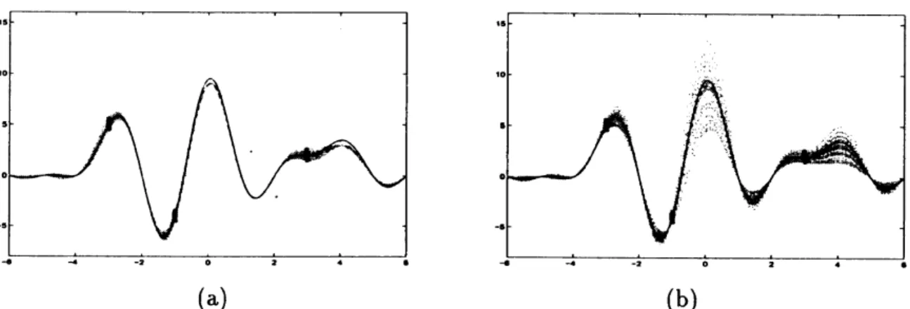
Figure2(a) and (b) show functionsobtained by minimum variance projection learning
and non-minimum variance SL projection learning, respectively, from thirty sets of
train-ing examples. They are shown by dotted lines. In both figures, $f(x)$ and $(Pf)(x)$ are also
shown by solid and dashed lines, respectively. These figures show that minimum variance
projection learning provides more stable results than other SL projection learnings
(a) (b)
Figure 2: Comparisonofminimum variance projection learning (MVPL) and non-MVPL.
(a) Resultant functions by MVPL from 30 sets oftraining examples, (b) Resultant
func-tions by non-MVPL from the same training examples as in (a).
6Conclusion
In this paper, we reviewed afunctional analytic theory of $\mathrm{s}\mathrm{u}\mathrm{p}\dot{\mathrm{e}}\mathrm{r}\mathrm{v}\mathrm{i}\mathrm{s}\mathrm{e}\mathrm{d}$ learning. First,
we formulated the problem of supervised learning by using areproducing kernel Hilbert
space. Then, projection learning, partial projection learning, and averaged projection
learning were introduced. Furthermore, these individual theories of learning were unified
into atheory of the family of projection learnings. It treats an infinite kind oflearning in
aunified way. By using the theory, we introduced minimum varianceprojection learning.
Model selection and active learning are also important topics in supervised learning.
The former is the problem of determining parameters in learning such as the subspace $S$,
while the latter is that of designing the sample points for optimal generalization. They
can also be discussed in this framework (see e.g. [11, 12]).
References
[1] Stefan Bergman, The Kernel Function and Conformal Mapping, American
Mathe-matical Society, Rhode Island, 1970.
[2] Akira Hirabayashi and Hidemitsu Ogawa, “Projection learning of the minimum
variance type,” In Proc. 1999 Int. Conf. on Neural Information Processing, vo1.3,
pp. 1172-1177, Perth, Australia, November 1999.
[3] Akira Hirabayashi and Hidemitsu Ogawa, “A family of projection learnings,” The
Transactions of the Institute of Electronics, Information and Communication
Engi-sets D-II, v0l.J83-D-II, n0.2, pp.754-767, February 2000 (in Japanese). Its short
English version titled “A class of learning for optimal generalization” appeared in
Proc. 1999 Int. Joint Conf. on Neural Networks, n0.246 (CD-ROM), Washington D.C., USA, July 1999.
[4] Hidemitsu Ogawa, “Projection filter regularization of ill-conditioned problem,” In
Proc. of SPIE, vo1.808, Inverse Problems in Optics, pp.189-196, March 1987.
[5] Hidemitsu Ogawa, “Inverse problem and neural networks,” In Proc. IEICE 2nd
Karuizawa Workshop on Circuits and Systems,pp.262-268, May 1989 (in Japanese).
[6] Hidemitsu Ogawa, “Neural networklearning, generalization and over-learning,” Proc.
ICIIPS’92, Int. Conf. onIntelligent Information Processing&System, Beijing, China,
Supplemental volume, pp.1-6, Oct. 1992.
[7] Hidemitsu Ogawa, “Neural networks and generalization ability,” The Institute of
Electronics, Information and Communication Engineers Technical Report,
n0.NC95-8, pp.57-64, May 1995 (in Japanese).
[8] Hidemitsu Ogawa and Shoji Hara, “Properties of partial projection filter,” The
Transactions of the Institute of Electronics, Information and Communication
Engi-neers A, vol.J71-A, n0.2, pp.527-533, February 1988 (in Japanese).
[9] Hidemitsu Ogawa and Kazutaka Yamasaki, “Generalization and over-learning of
neural networks,” The Institute of Electronics, Information and Communication
Engineers Technical Report, no.NC91-75, pp.77-84, January 1992 (in Japanese).
[10] Robert Schatten, Norm Ideals of Completely Continuous Operators,
Springer-Verlag, New York, 1970.
[11] Masashi Sugiyama and Hidemitsu Ogawa, “Incremental active learning for optimal
generalization,” Neural Computation, vo1.12, n0.12, pp.2909-2940, December 2000.
[12] Masashi Sugiyama and Hidemitsu Ogawa, “Subspace information criterion formodel
selection,” Neural Computation, vo1.13, n0.8, pp.1863-1889, August 2001.
[13] Sethu Vijayakumar, Masashi Sugiyama, and Hidemitsu Ogawa, “Training data
se-lection for optimal generalization with noise variance reduction in neural networks,”
In Proc. WIRN Vietri-98, The 10-th Italian Workshop on Neural Nets, pp.153-166,
Salerno, Italy, May 1998.
[14] Yukihiko Yamashita and Hidemitsu Ogawa, “Properties of averaged projection filter
for imagerestoration,” The Transactions of the Instituteof Electronics, Information
and Communication Engineers D-II, v0l.J74-D-II, n0.2, 142-149, February 1991
(in Japanese). Its English translation appeared in Systems and Computers in Japan,
Scripta Technica, Inc. USA, vo1.23, no.1, pp.69-78, April 1992