Execution and verification of 2nd order interval temporal logic(Concurrency Theory and Applications '96)

Execution

and

verification of

2nd order

interval

temporal

logic

Shinji

Kono

$\mathrm{e}$

-mail:[email protected]

Sony

Computer

Science

Laboratory

Inc.

3-14-13,

Higashi-gotanda,

Shinagawa-ku, Tokyo 141,

Japan

November 16, 1995

Process is the value of second order interval propositional temporal logic ($2\mathrm{I}\mathrm{T}\mathrm{L}$here

after). Not only temporal relation-ship

among

events, but also

processes

are

directly

defined interms oftemporal logic. Since it

can

express

a

negation of

a

process, it

covers

different

range

from process algebra. Process includes finite state machine, fairness,

a

scheduling mechanism, inverse specification, and various temporal logicformula. In this

paper

we

show $2\mathrm{I}\mathrm{T}\mathrm{L}$

as a

subset of interval temporal logic. $2\mathrm{I}\mathrm{T}\mathrm{L}$ is undecidable, but

through investigations

on

verification procedures,

we

find decidable subset of ITL. Its automatic verificationis also presented.

1

Interval Temporal

Logic

as

Second

Order

Temporal

Logic

Interval temporal logic (Ref. [12] ITL here after) is investigated by various researchers, but because of its undecidability (Ref. [12]), researches

are

restricted

on

Local Interval Temporal Logic (Local ITL here after). In Local ITL, variables represents events depending

on

a

clock period like other

Temporal Logics. On the other hand, variables of full set ITL represent series of events in intervals

oftime. We

can

think the variablesrepresent processes since it includes possibly

an

infinite stream

of events. This is

a

new

view point ofITL, that is

a

logic

on processes.

In

case

of classical logic, second order propositional logic is trivial, because the value of the

second order variable is either $T$

or

$F$. There

are

no

differences between second order logic and

normal logic. But in

case

oftemporal logic, value of second order variable is changed from time to time. It looks like first order logic, but the value of the variable is not

a

return value of

a

function,

which is determined by arbitrary nested function calls. First order logicis undecidable because first

order value

can

be arbitral nested term. But the value of the second order propositional variable is restricted in the meaning of the temporal logic, which

can

be

a

finitely represented state machine.

Like

a

first order logic

on

enumerable term,

a

second order temporal logic

can

be decidable.

2Expressiveness of

Various

Temporal

Logic

After the discovery of

a

limitation of Linear Time Temporal Logic (LTTL here after. Ref. [13]),

complex hierarchy of temporal logic expressiveness is researched. A big surprise is that LTTL is

less expressive than $\omega$-Regular expressions

on

logic

formula.

We

can

prove similar limit

on

Local

ITL (Appendix). But

we

find such

a

limitation is not serious.

The limit is easily solved by adding quantifier

or

adding closure operation

on

logics. Quantified

Propositional TemporalLogichas $\omega$-Regular model(Ref. [13]). Actually it isquite

easy

to construct

a

representation of arbitrary finite state machine (here after FSM) using quantified variables. We

can

use

quantified variables for 1-hot encoding of

a

FSM (Ref. [9]). A closure $\mathrm{o}\mathrm{p}\mathrm{e}\mathrm{r}\mathrm{a}\mathrm{t}\mathrm{o}\mathrm{r}*\mathrm{i}\mathrm{s}$ also

sufficient to construct

a

FSM by using well-known algorithm

on

Regular Expression (Ref. [7]). A

closure $\mathrm{o}\mathrm{p}\mathrm{e}\mathrm{r}\mathrm{a}\mathrm{t}\mathrm{o}\Gamma*P$

means

finite

or

infinite repetition of

a

temporal logic formula$\cdot$

$P$

.

This is easily

demonstrated by

an

example called evenp.

evenp$(p)$

means

$P$ is true

on every even

clock period. We

use

small letters _$p,$$q,$$r$ for event

variables. In Regular Expression, $(\mathrm{P}\mathrm{T})*$. It is proved evenp_$(p)$ is not expressed in LTTL

nor

Local ITL (Appendix). But it is easily expressed by QPTL; evenp$(p)\equiv\exists q,$$q$A $\square$ (

$(qarrow \mathrm{O}\neg q)$ A $(\neg qarrow \mathrm{O}q)$ A _{$qarrow p$}).

It is also easily expressed by closure $\mathrm{o}\mathrm{p}\mathrm{e}\mathrm{r}\mathrm{a}\mathrm{t}\mathrm{o}\mathrm{r}*\mathrm{l}\mathrm{i}\mathrm{k}\mathrm{e}$this;

evenp$(p)\equiv*$((($p$ A length(l))&length(l)) Vempty).

&is a

chop operator which is

one

clock overlapped concatenation of two intervals. Intervals

are

finite

or

infinite clock period.

P&Q

$\mathrm{P}$

$\mathrm{Q}$

empty

means

the length of the interval is $0$.

$\mathrm{e}\mathrm{m}\mathrm{H}^{\mathrm{P}^{\mathrm{t}\mathrm{y}}}$

But

on

theseextenslons, verltications

on

thelogicrequlres exponential computationalcomplexity

on

the length offormula. Polynomial order

or

lower complexity is preferable of course, but recent

researches

on

BDD based verification (Ref. [2]) show

we can

still verify useful examples

even

in

case

of exponential computational complexity, if

we

takes enough effort to keep state

space

representation small.

From the view point of automatic verification, closure operator is superior. Because quantifier

generates exponential computation

on

number ofvariables, which corresponds number of edge of

states. Even classicalpropositional quantified logic requires $\mathrm{P}$-spacecomplexity. In

case

ofclosure,

it generates exponential computation

on

depth oftemporal logic operator, which increases number

3Expressiveness

and

Decidability

of Interval

Temporal

Logic

ITL and LTTL both feature discrete time, but ITL has the end of the time. Unlike LTTL, ITL

has

a

model

on

top of Regular expression not

on

top of$\omega$-Regular expression. In another words,

ITL has compact discrete time. It has pros and

cons.

ITL cannot

express

fairness like LTTL. For

example, $\square \mathrm{O}p$ does not

means

_$p$ is true infinitely many times but it

means

_$p$ is true

on

the end of

the

_{interval.. In.}

$\mathrm{f}\mathrm{a}\mathrm{c}\mathrm{t}\wedge\cdot’$

.

$\square \dot{\mathrm{O}}Prightarrow fin(P)$

is

a

theorem in Local ITL. Here

we use

capital letter $P,$ $Q,$$R$ (other than $F$ and $T$) forsecond order

variable

or

interval variable. Here

_fin

$(P)$

means

$P$ is true

on

the end of the interval and these

are

defined in Local ITL

using&as

follows; ’

fin

$(P)$ $\equiv$ (T&(empty A $P$))

$\square P$ $\equiv$ $\urcorner(T\ \urcorner P)$

$\mathrm{O}P$ $\equiv$ T&P

The theoremis not trivial but it is easy to prove and it

means

the lack offairness in Local ITL. But this makes

a

verification procedure easier, because

we

don’t have to check state loop after tableau expansion

as

in M\"uler _{automaton. If}

_we

_have

_no

_false

_on

the leaves of the FSM, the formula is valid.

Now

we

know Local ITL with closure has Regular Expression expressiveness. We also have

a

FSM generation algorithm for Local ITL with closure (Ref. [9]). This shows

Theorem 1 Local $ITL$

wit.h.

closure has exact Regular Expression expressiveness.

In

case

of full ITL, things

goes

badly. It is quite

easy

to show ITL

can

express Context Free

Grammar and Context Dependent Grammar. An interval variable contains

a

series ofstates which

is

a

mapping of event variables. We

can

use an

event variable mapping

as

a

terminal symbol and

an

interval variable

as a

non-terminal symbol in

grammar

rule. For example,

means a

context dependent

grammar

rule: $PQarrow RS$. Here a $P$

means

a

formula $P$ is true in all

sub-intervals ofthe interval. It is defined

as

follows;

$\mathrm{a}(P)\equiv$

\neg (T&\neg P&T).

This is rarely used in Local ITL specification, but important in $2\mathrm{I}\mathrm{T}\mathrm{L}$. Since satisfiability problem

on

Context Dependent Grammar is undecidable, full ITL is also undecidable. This is another proof

$\mathrm{o}\mathrm{f}[12]$.

Theorem 2 Full $ITL$ is undecidable.

But closer look of this problem gives

us

another insights. S. Kimura shows the undecidability

of ITL

comes

from interval variable itself (Ref. [8], in Japanese). An interval variable

can

be

instantiated with

an

arbitrary finite

or

infinite sequence, which includes

a

sequence generated by

a

context dependent

grammar.

This is the

source

ofundecidability. $\mathrm{W}\mathrm{e}’ 11$ investigate this problem

Local variables

or

events

are

restricted form of interval variable, which has the

same

value

on

empty interval of the beginning of the interval. This restriction makes ITL decidable, it is Local

ITL. Locality of$P$ is characterized by next proposition;

beg(P)\leftarrow \rightarrow P&T

where $beg(P)=$ (($\mathrm{e}\mathrm{m}_{\mathrm{P}^{\mathrm{t}\mathrm{y}}}$,P)&T). But

we

can

think another restriction

on

it.

If

we

restrictinterval variables

can

be instantiated by RegularExpression generated sequence,

we

have Regular ITL instead ofLocal ITL. Unfortunately Regular ITL is still undecidable. Remember

we

can

express Context Free Grammar (here after CFG) in ITL. We

can

construct

an

ITL formula

which checks

a

CFG is Regular

or

not. For

a

given CFG, construct ITL formula, for example,

$P\wedge \mathrm{a}c_{ramm}er(P)$. If this is satisfiable in Regular ITL, the CFG is Regular. It is known that

whether

an

context free

grammar

is Regular

or

not isundecidable (Ref.[7]). So there is

no

_proced.

ure

to check whether Regular model for ITL exists

or

not.

Theorem 3 Regular $ITL$ is undecidable.

In this paper, $\mathrm{w}\mathrm{e}’ 11$ show

some

other restrictions which makes ITL decidable. The most simple

one

is length restriction. These restrictions defined in terms of tableau expansion. In

some

sense, it

can

be called operational restriction of interval variables. These restrictions

are

model restrictions.

In

case

of verification

on

first order logic, they

use

incomplete decision procedure. It will not

terminate

or

$\mathrm{t}\mathrm{e}\mathrm{r}\mathrm{m}^{l}\mathrm{i}\mathrm{n}\mathrm{a}\mathrm{t}\mathrm{e}$ but gives incomplete results. Our logic is

sound and complete in terms of

automatic verification procedure. But completeness is defined

_{rather.ad-hoc}

way which is defined

in operation in the tableau method.

This is something like

a

restriction

on

programming methodology. We

can

program

anything

on

Turing Machine, but not all the

program

is good

one.

If

we use a

restricted programming method,

we

can

extend reliability of the

program.

The restrictions of interval variables

are

thought

as

such restrictions. Since it is

a

restriction

on

second ordervariables, the expressiveness ofthe logic is still equivalent to Regular Expressions. This corresponds the fact that

a

programming methodology

does not restrict the power of programming.

4

Specification Examples

Since

a

second order variable represents

a

mechanism to terminate

an

interval, it is possible to

think it

a

fairness.

$\mathrm{O}_{S}P\equiv S\ P$

$\mathrm{O}_{S}P$

means

$P$ is eventually true

on

fairness $S$, eventuality-S. Unlikefairness in LTTL,

many

kinds

of different fairness

can

be defined in $2\mathrm{I}\mathrm{T}\mathrm{L}$. In fact the value of second order variable is different

on

each clock period,

so

it defines different fairness

on

each clock period. To define clock period independent fairness,

a

time constant second order variable is

necessary.

We discussit later section.

We

can

think this is

an

abstraction of watch dog timer

or

counter. The mechanism of the timer

can

be defined in terms ofITL;

$\mathrm{a}(S=leSS(2))$

This

means

$S$

assures

an

interval which is less than 2 clocks. less_$(n)$ operator

can

be defined

using $\mathrm{n}$-times nested weak next operator; less(2)

$\equiv \mathrm{O}\mathrm{O}\mathrm{e}\mathrm{m}_{\mathrm{P}^{\mathrm{t}\mathrm{y}}}.\cdot$ This is

a

simple watch dog timer

For another example, using second order variables,

we can

directly prove axiom schema. Our

verifier is based

on

model construction,

so we

can

verify

some

axioms. For example;

$\mathrm{a}((\mathrm{a}(P)arrow P))arrow(((\Phi(\mathrm{a}(P)))arrow \mathrm{a}(P)))))$.

This is called $\mathrm{Z}$ discreteness (Ref. [5]). Thisis valid in LTTL, but not valid in ITL.

Of course,

we can use

second ordervariablestodefine

a

processby recursion like process algebra.

$\mathrm{a}(Parrow$ ($(a$ A $\mathrm{O}P)\vee(b$A $\urcorner a\wedge$ empty))

But

we

have to consider the $\mathrm{r}\mathrm{e}\dot{\mathrm{s}}$

trictions of second order variables in these process representations

in

case

of verification.

If

we

try to write

a

practical specification in temporallogic, it isusually

non

valid formula

even

if

we

quantified all variables. This is because there

are

hidden assumptions

on

input variables. These

assumptions

can

be abstracted using second order variables. Using the result of tableau expansion,

we can

analyze the nature ofthe assumption. In

some sense

this is kind of

reverse

specification.

5

Undecidability from

a View Point

of Tableau

Expan-sion

In this section,

we

discuss

on a

tableau method of$2\mathrm{I}\mathrm{T}\mathrm{L}$. In Tableau method

on

discrete temporal

logic, temporal logic terms

are

decomposed into two parts. One part is depending only

on

current clock period and the other part only depends

on

next

or

later interval.

Here

we

show

an

example of decomposition of

a

chop operator. Assume $P,$$Q$ is already

de-composed into empty parts $PE,$ $QE$, current clock dependent parts $PN_{i},$$QN_{i}$ and next interval

dependent parts $PX_{i},$ $QX_{i}$ in disjunctive normal form.

$P$ $=$ $PE$ Aempty$\vee\bigvee_{i=0}^{k}$($PNi$ A _{$@PX_{i}$})

$Q$ $=$ $QE$ Aempty $\bigvee_{i=0}^{k}$($QNi$ A _{$@QX_{i}$})

Where @ is next operator with $\neg \mathrm{e}\mathrm{m}\mathrm{p}\mathrm{t}\mathrm{y}$ and it is called strong next. Then

P&Q

is decomposed in

this way.

P&Q

$=$ $(PE\wedge Q)\vee$

$\mathrm{V}_{i=0}^{k}$($PNi$ A $@(PX_{i}\ Q)$)

In practical tableau expansion, BDD standard form and deterministic expansion is necessary, but

these

are

discussed in (Ref. [4, 3, 9]).

In

case

of second order variable

or

interval variable, the value of the variable is depend

on

the

both begin-time and end-time of the interval. Since

we

are

working

on

propositional case, it looks

like

we can

replace the value of the variable by $T$

or

$F$. Yes, the value is $T$

or

$F$, but the value

depends

on

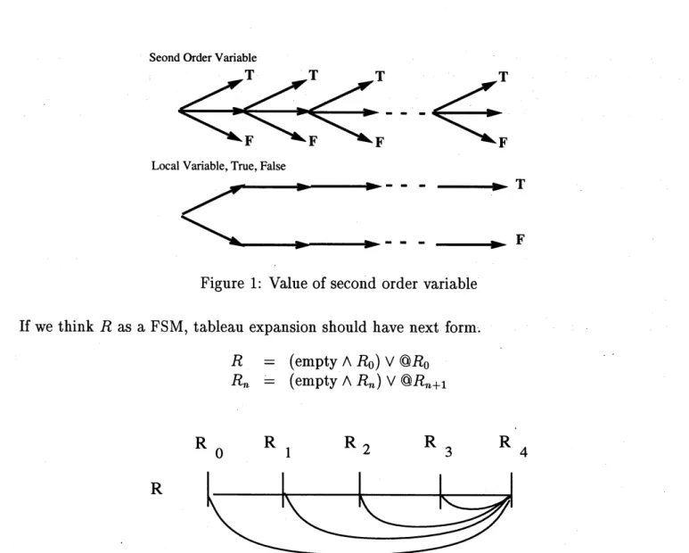
the interval (Fig. 1). So

we

cannot replace the second order variable with $T$

or

$F$

as

we

did in classical logic.

This situation is demonstrated by

an

example:

$\mathrm{a}(R=length(2))$

If

we

replace $R$ by $T$

or

$F$, this example becomes unsatisfiable. But this is satisfiable if

we

$\mathrm{S}\mathrm{e}\circ^{\mathrm{n}A\mathrm{n}\mathrm{P}}A\mathrm{a}\mathrm{P}1\gamma_{\mathrm{Q}\dot{\mathrm{r}}}\mathrm{o}\mathrm{h}\iota\wedge$

LocalVariable, True,False

$-arrow \mathrm{T}$

$-rightarrow \mathrm{F}$

Figure 1: Value of second order variable If

we

think $R$

as a

FSM, tableau expansion should have next form.

$R$ $=$ $(\mathrm{e}\mathrm{m}\mathrm{p}\mathrm{t}\mathrm{y}\wedge R_{0})@R_{0}$

$R_{n}$ $=$ $(\mathrm{e}\mathrm{m}\mathrm{p}\mathrm{t}\mathrm{y}\wedge R_{n})\vee@R_{n+1}$

$\mathrm{R}0$ $\mathrm{R}1$ $\mathrm{R}2$ $\mathrm{R}3$ $\mathrm{R}4$

$\mathrm{R}$

$R_{n}$ is n-th state of R. $R_{n}$ is also

a

second order variables. $R_{n}$ is independent each other if _$n$ is

different. This is because $R_{n}$ has different start point and $R$ has different truth value in different

interval. Using existential quantifier

on

second order variable,

we can

write;

$R$ $=$ $(\mathrm{e}\mathrm{m}\mathrm{p}\mathrm{t}\mathrm{y}\wedge R)\vee@$ $\exists SS$.

During the tableau expansions, $n$ increases infinitely. Actually $n$ represents the interval length of

$R$. In

case

of

a

formula like $\square R$, infinitely many $R_{n}$

are

generated. In this way, undecidability of

full ITL

or

$2\mathrm{I}\mathrm{T}\mathrm{L}$ happens in the tableau expansion.

Projection operator and quantifier

on

second order variables is not considered in this paper.

Since projection operator requires

a

nest time structure, the time marking of$R$ have to be

a

nested

markings. It looks like possible to implement it, but

we

have not yet tested yet.

5.1

Length

Restriction

and

Count Restriction

The simplest stopper of the undecidability is length limit.

$R$ $=$ $\mathrm{e}\mathrm{m}\mathrm{p}\mathrm{t}\mathrm{y}\wedge R_{0}\wedge@R_{0}$

$R_{n}$ $=$ $\mathrm{e}\mathrm{m}\mathrm{p}\mathrm{t}\mathrm{y}\wedge R_{n}\wedge@R_{n+1}$ if $n<k$

$R_{n}$ $=$ $beg(Rn)\mathrm{i}\mathrm{f}n\geq k$

$R_{n}$ is generated

on

every

clock. But if

we

have only

one

$R_{n}$,

we

don’t have to

use

specific $n$.

Any other number is also $\mathrm{o}\mathrm{k}$. We

can

compact the number

sequence

by sort and renaming. But

the order of the number have to be preserved. After renaming, $n$ represents number of $R_{n}$ in

a

formula. We

can

call this restriction count limit. The count limit is useful

on a

formula like this:

R&T.

In this example, $R_{n}$

increases

$n$ by 1. This generates

a

series like this.

R&T,

$R_{1}\ \tau,$$R_{2^{\ T,\ldots R_{n}\ T}}$

If

we

think $R$ and $R_{1}$

are

equivalent, this example is expanded to itself. Roughly speaking,in count

limit method,

we

have

no

limit

on one

time R-eventuality.

5.2

More

Complex

Restrictions

But above restrictions does not work well

on

a

formula like T&R that is OR. In this example, expanded formula has

a

form after $n$ clocks;

$R_{0}R_{1}$ V... V $R_{n}\vee T\ R.$

After $R_{n}$ reaches the limit, it becomes $T$

or

$F$. In this case, renaming of $R_{n}$ becomes identity

and useless. Looking at the formula carefully,

we

find every $R_{n}$ exists only

once.

The meaning of

this formula is not depends

o

$\mathrm{n}$

- the particular

name

of

$R_{n}$ and $R_{n}$ is independent each other. It is

possible to

remove

$R_{n}$ from the formula. This is called singleton removal.

Singleton removal is possible and it extends possible meanings of second order variables. But

currently

we

have rather complex translation of the formula which generates alot of states. Besides

even

after the singleton removal, $R$ still possible to generate increasing complex logical expressions

on a

formula with multiple

occurrence

of$R_{n}$. $2\mathrm{I}\mathrm{T}\mathrm{L}$is of

course

undecidable with singleton removal.

Singleton removal is not practical because it $\mathrm{g}\mathrm{e}\mathrm{n}\sim$erates big state space. In this reason,

we

don’t

investigate singleton removal further

h\‘ere.

Here

we

show several restriction methods

on

decidable $2\mathrm{I}\mathrm{T}\mathrm{L}$;

length limit Effects of$R$ has time $\mathrm{l}\mathrm{i}\mathrm{n}\dot{\mathrm{u}}\mathrm{t}$,

count limit Number of $R$ is limited,

singleton removal Number of interrelated $R$ is limited.

These

are

defined in

an

operational way in the tableau expansion.

To make $2\mathrm{I}\mathrm{T}\mathrm{L}$ decidable, finiteness of $2\mathrm{I}\mathrm{T}\mathrm{L}$ term is necessary. What

we

need is define finite

classification of subset of $R_{n}$. Here

we

intr.o

$.$

$\mathrm{d}$

uce

some

of simple classifications, but there

can

be

more

useful classifications. ..

Computational complexity of $2\mathrm{I}\mathrm{T}\mathrm{L}$ verification is determined by the restriction. Local ITL

verification requires exponential complexity of the length ofthe formula, that mostly

comes

from

determination of expanded states. In the worst case, all combination of the sub terms have to be

computed. $R_{n}$ terms increase the number the sub term,

as

result in effect of $2^{n}$. In

our

experience,

6Execution

of 2nd

Order Interval

Temporal

Logic

In the tableau expansion based verification (Ref.[9]),

a

deterministic FSM is generated. This is

a

method of logic synthesis

or program

generation.

$-$

In

case

of$\mathrm{L}_{\mathrm{o}\mathrm{C}}\mathrm{a}1$

.ITL, all variables

are

events. An

execution of the FSM is something like flipping traffic rights.

An execution of $2\mathrm{I}\mathrm{T}\mathrm{L}$ is not

so

simple. Besides conditions

on

events

variable, it also contains

conditions

on

second order variables. The conditions $\mathrm{d}\mathrm{e}\mathrm{p}\mathrm{e}\mathrm{n}\mathrm{d}_{\mathrm{o}\mathrm{n} ,-}$the restriction methods.

Length limit is the most simple

one.

It contains two kind of events

on

$R$.

termination $R$ is terminated in $T$

or

$F$ in less than length _$n$ interval.

time out the limit of $R$ expired and results $T$

or

$F$.

These

are

marks

on

the FSM and define FSMs for $R$

on

each clock period. It also define

a

trace of

$R$ in the execution.

In

case

of count limit,

we

have to consider renaming of $R_{n}$. Other

situation

is similar to the

length limit

case.

Therenaming is assignedto each transitionin thegeneratedFSM. Using renaming

information,

we can

find

a

FSM definition of$R$

on

each clock period.

Since

we

omit the detail ofsingleton removal,

we

cannot discuss execution in singleton removal,

here.

7

Time

Constant

Second

Order Variable

In $2\mathrm{I}\mathrm{T}\mathrm{L}$,

a

FSM assigned to

a

second order variable is varied

on

the interval. If

we

assign

one

fixed

FSM

on

the variable,

we

have time constant second order variable.

_The.effect

of the assignment

can

be represented usin$\mathrm{g}$

- ITL formula, for example,

$\mathrm{a}(R=leSS(2))$.

If there is

a

model for time constant second order variable, there must be

a

model for

non

time constant variable. For particular execution

path:

we can

easily check if

some

of $R$ traces

are

conflicted. But currently

we

have

no

method to find out constant FSM for $R$.

8

Execution and Verification Examples

In this section,

we

see

actual output of

our

verifier, which is written in Prolog.

8.1

Example: Length

Operator

and

Second Order Variable

We

can

demonstratethe difference oflengthlimit and countlimit byusingsimple example: $R\wedge(R=$

$length(10))$_{. Here}

we assume

_{limit is 5. length(10) is expressed by nested strong next operator and}

this becomes the first state.

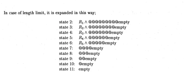
In

case

of$\mathrm{l}\mathrm{e}\mathrm{n}$

.gth limit, it is expanded in this

way;

state 2: $R_{1}$ A @@@@@@@@@empty state 3: $R_{2}$ A @@@@@@@@empty state 4: $R_{3}$ A @@@@@@@empty state 5: $R_{4}$ A @@@@@@empty state

6:

$R_{5}$ A @@@@@empty state

7:

@@@@empty state 8: @@@empty state 9: @@empty state 10: @empty state 11: empty

In state 5, $R_{6}’ \mathrm{s}$ truth value is fixed. $R_{6}$ is false entire formula is false otherwise @@@@empty

remains. The resulted state diagram is show in (Fig.2). Using this FSM,

we can

find executions.

An execution is shown like this.

LengthLimit

Kenamung $A\wedge\cdot\cdot,\mathrm{r}’\prime 1\backslash$

Figure 2: FSM for Length Example

$|?-$ ex$((^{\wedge}\mathrm{r}, (\mathrm{l}\mathrm{e}\mathrm{n}\mathrm{g}\mathrm{t}\mathrm{h}(10)=\wedge \mathrm{r})))$

.

0.46299999999999963 sec. 11 states 16 subterms 23 state transitions counter example: $0:+\mathrm{r}^{\wedge}0$ false $|?-\mathrm{e}\mathrm{x}\mathrm{e}$

.

execution: $0:2$ 1: 3 2: 4 3: 5 4: 6 $5:+_{\mathrm{O}}\mathrm{v}\mathrm{e}\mathrm{r}(\mathrm{r},5^{)}7$ 6: 8 7: 9

8: 10 9: 11 10: $0$

yes

$\wedge \mathrm{r}$ is the second order variable notation in

our

verifier. The first number is clock value and

second is the number of state. $+_{\mathrm{O}\mathrm{V}\mathrm{e}\mathrm{r}}(\mathrm{r},5)$

means

$R_{5}$ is reached the limit and fixed to $T$ and this

is

a

transition condition of the FSM.

In

case

of count limit,

we

have renumbering of $R_{n}$. The FSM and execution is shown below.

$+\mathrm{r}^{\wedge}1$

means

$R_{1}$ is$T$ in theempty interval at the clock. This result looks

more

correct thanprevious

one.

state 2: $R_{1}\wedge@@@@@@@@@\mathrm{e}\mathrm{m}\mathrm{P}\mathrm{t}\mathrm{y}$ state 3: $R_{1}\wedge@@@@@@@@\mathrm{e}\mathrm{m}_{\mathrm{P}^{\mathrm{t}}\mathrm{y}}$ state 4: $R_{1}\wedge@@@@@@@\mathrm{e}\mathrm{m}_{\mathrm{P}^{\mathrm{t}}\mathrm{y}}$ state 5: $R_{1}\wedge@@@@@@\mathrm{e}\mathrm{m}\mathrm{P}\mathrm{t}\mathrm{y}$ state 6: $R_{1}\wedge@@@@@\mathrm{e}\mathrm{m}\mathrm{P}\mathrm{t}\mathrm{y}$ state

7:

$R_{1}\wedge@@@@\mathrm{e}\mathrm{m}\mathrm{P}\mathrm{t}\mathrm{y}$ state 8: $R_{1}\wedge@@@\mathrm{e}\mathrm{m}\mathrm{P}\mathrm{t}\mathrm{y}$ state 9: $R_{1}\wedge@@\mathrm{e}\mathrm{m}\mathrm{P}\mathrm{t}\mathrm{y}$ state 10: $R_{1}\wedge@\mathrm{e}\mathrm{m}_{\mathrm{P}^{\mathrm{t}\mathrm{y}}}$

state 11: $R_{1}\wedge \mathrm{e}\mathrm{m}\mathrm{p}\mathrm{t}\mathrm{y}$

$|$ $?-$ ex((

$\mathrm{r}$, (length(10) $=\wedge \mathrm{r}$))).

0.5179999999999998 sec. 11 states. 12 subterms 23 state transitions

yes

$|?-\mathrm{e}\mathrm{x}\mathrm{e}$

.

execution: $0:2$ 1: 3 2: 4 3: 5 4: 6 5: 7 6: 8 7: 9 8: 10 9: 11 $10:+\mathrm{r}1- 0$

In above examples, limit has

no

effect

on

verification. We have 5 clock limit

on

$R$, but it does

not restrict the length of the interval. The limit restrict the behavior of the variable. The verifier

$R$A $\mathrm{a}(length(4)=R)$ is such example. We

can

write expanded state in

a

simplified

way;

state 2: $R\wedge \mathrm{a}(length(4)=R)\wedge$

($R_{1}$ A

:

(length(3) $=R_{1})\ T$)

state

3:

$R$A $\mathrm{a}(length(4)=R)\wedge$

$(R_{1}\wedge:(length(3)=R_{1})\ T)\wedge$

$(R_{2}\wedge:(length(2)=R_{2})\ T)$

state 4: $R\wedge \mathrm{a}(length(4)=R)\wedge$

$(R_{1}\wedge \mathrm{i}(length(3)=R_{1})\ T)\wedge$

($R_{2}$ A

:

(length(2) $=R_{2})\ T$)$\wedge$

$(R_{3}\wedge:(length(1)=R_{3})\ T)$

state 5: $R\wedge \mathrm{a}(length(4)=R)\wedge$

($R_{1}$ A

:

(length(3) $=R_{1})\ T$)$\wedge$

$(R_{2}\wedge \mathrm{i}(length(2)=R_{2})\ T)\wedge$

($R_{3}$ A

:

(length(1) $=R_{2})\ T$)$\wedge$ $(R_{4}\wedge \mathrm{i}(length(\mathrm{O})=R_{4})\ T)$

Here $\mathrm{i}R\equiv\neg(\neg R\ T)$. In this example, a is decomposed by $\mathrm{i}$ .

a$Prightarrow\square$

:

$R$.

The generated FSM is executed in

length4-

interval

as we

expected.

$|$ $?-$ ex(( $\mathrm{r}$, ’ $[\mathrm{a}]$ ’(length(4) $=\wedge \mathrm{r}$))).

2.362 sec. 7 states 18 subterms 15 state transitions yes $|?-\mathrm{e}\mathrm{x}\mathrm{e}$

.

execution: $0:-\mathrm{r}^{\wedge}02$ $1:-\mathrm{r}^{\wedge}$0-rl- 3 $2:-_{\mathrm{r}^{\wedge}0-_{\mathrm{r}^{\wedge}12}}-_{\mathrm{r}}\wedge 4$ $3:-\mathrm{r}^{\wedge}0^{-}\mathrm{r}1--\mathrm{r}2--\mathrm{r}3\wedge 5$ $4:-\mathrm{r}^{\mathrm{s}}0-\mathrm{r}arrow 1-\mathrm{r}^{\wedge}2-_{\mathrm{r}3+}- \mathrm{r}^{\wedge}40$

yes

$-\mathrm{r}^{\wedge}\mathrm{n}$

means

$R_{\tau\iota}$ is $F$ at the clock period $\mathrm{a}\mathrm{n}\mathrm{d}+_{\mathrm{r}^{arrow}}\mathrm{n}$

means

$R_{n}$ is $T$.

Of

course

we can

prove

a

theorem like this;

$\mathrm{a}(R=lesS(\mathit{3}))arrow((R\ R\ R)arrow lesS(\mathit{9}))$.

The length limit is working

on

each $R$ and

a

complex term like (R&R&R)

can over

$\mathrm{c}\mathrm{o}\mathrm{m}$

. $\mathrm{e}$ the limit

with extra computation. This is because only

one

$R$ is active at each clock.

$|?-$ ex((’ $[\mathrm{a}]$ ’ ( $\mathrm{r}=$ less(3)) $-\rangle((^{\wedge}\mathrm{r}$ & $\wedge \mathrm{r}$ & $\wedge \mathrm{r})-\rangle$ less(9)))).

27.989999999999995 sec. 100 states 35 subterms 629 state transitions valid yes

The execution of this formula is not interesting because this is

a

theorem. It succeeds in any

interval. To

see an

interesting one;

$|?-$ ex((’ $[\mathrm{a}]$ ’ ( $\mathrm{r}=$ less(3)) , $((^{\wedge}\mathrm{r}$

a

$\wedge \mathrm{r}$

a

$\wedge \mathrm{r}))$)).

2.519999999999996 sec. 15 states 29 subterms 37 state transitions yes $|?-$ exe(7). $0:+\mathrm{r}^{\wedge}0$ 2 $1:+_{\mathrm{r}^{\wedge}}0+\mathrm{r}^{\wedge}1$ 3 $2:+_{\mathrm{r}^{\wedge}}\mathrm{o}+_{\mathrm{r}}1- \mathrm{r}^{\wedge}+2$ 4 $3:+_{\mathrm{r}^{\wedge}}0+\mathrm{r}^{-}1+\mathrm{r}^{-}2^{-}\mathrm{r}arrow 3$ 5 $4:+\mathrm{r}^{\wedge}\mathrm{o}+_{\mathrm{r}}\wedge 1+\mathrm{r}^{arrow}2-_{\mathrm{r}\mathit{3}4}--\mathrm{r}^{\wedge}$ 6

$5:+\mathrm{r}0-+_{\mathrm{r}^{arrow}1}+\mathrm{r}arrow 2^{-}\mathrm{r}^{\sim}\mathit{3}-\mathrm{r}^{-}4^{-\mathrm{r}^{\wedge}}5$-over(r,5) 8 $6:+\mathrm{r}0-- 1+\mathrm{r}+\mathrm{r}2^{-\mathrm{r}}-- 3-\mathrm{r}^{\wedge}4^{-\mathrm{r}^{\wedge}}5$ $0$

yes

Clearly $\wedge \mathrm{r}$ is $T$ in each interval which length is less than 3 and $F$ otherwise.

As

an

example of limitation, $R$A $\mathrm{a}(length(10)=R)$ is unsatisfiable if

we

have length limit 5

or

count limit 5. Since this example contains T&R type expression, there

are no

big

difference

between length limit and count limit.

$|?-$ ex(( $\mathrm{r}$, ’ $[\mathrm{a}]$ ’ (length(10) $=\sim_{\mathrm{r})})$).

3.2110000000000003 sec. 7 states 24 subterms 14 state transitions yes $|?-\mathrm{e}\mathrm{x}\mathrm{e}$

.

execution: unsatisfiable

8.2

Example:

$\mathrm{Z}$

discreteness and Diodorean discreteness

Diodorean discreteness (Ref. [5]) is

$\mathrm{a}(\mathrm{a}(((Rarrow \mathrm{a}R)arrow R)))arrow\phi\iota\iota Rarrow \mathrm{a}R$.

We

can

easily

prove

it under the count limit restriction.

$?-$ ex$(’[\mathrm{a}] ’ (’[\mathrm{a}] ’ (((^{\wedge}\mathrm{r}^{-}>’[\mathrm{a}] ’ (^{arrow}\mathrm{r}))->\wedge \mathrm{r})))->’<\mathrm{a}>’(’[\mathrm{a}] ’ (^{\wedge}\mathrm{r}))->)[\mathrm{a}]$’ $(^{arrow}\mathrm{r}))$

.

15 states

24 subterms

98 state transitions

valid yes

In

case

of $\mathrm{Z}$ discreteness;

$\mathrm{a}((\mathrm{a}(R)arrow R))arrow(((\Phi(\mathrm{a}(R)))arrow \mathrm{a}(R)))))$.

We have counter example.

$?-$ ex(’ $[\mathrm{a}]$ ’((’ [al ’ $(^{\wedge}\mathrm{r})->\wedge \mathrm{r}))->’<\mathrm{a}>$ ’ (’ $[\mathrm{a}]$ ’ $(^{arrow}\mathrm{r}))->’[\mathrm{a}]$ ’ $(^{\wedge}\mathrm{r})$).

30.710000000000008

sec. 23 states 24 subterms 149 state transitions counter example: $0:+_{\mathrm{r}^{\wedge}}0$ 2 $1:+_{\mathrm{r}^{\wedge}}0-\mathrm{r}^{arrow 1}$ false

8.3

Example:

Grammar Rules or Recursive Process

A $2\mathrm{I}\mathrm{T}\mathrm{L}$formula,

$R\wedge \mathrm{a}$ ($(Rarrow((a$ A @R) V $(\neg a\wedge b\wedge \mathrm{e}\mathrm{m}\mathrm{p}\mathrm{t}\mathrm{y})))$)

represents

a grammar

rule

or

$\mathrm{C}$CS like

process.

But

we

are

using discrete time and it

use

$\mathrm{a}$

operator, the verifier generates rather big FSM.

$|?-$ ex(( $\mathrm{r},$ ’ $[\mathrm{a}]$ ’ (( $\wedge \mathrm{r}-\rangle$ (($\mathrm{a}$,@ $\wedge \mathrm{r}$) $;(^{\sim}\mathrm{a},\mathrm{b}$,empty)))))).

76.817 sec. 128 states 22 subterms 264 state transitions yes $|?-$ exe(5). $0:+\mathrm{a}^{-_{\mathrm{r}^{-}0}}3$ $1:+\mathrm{a}^{-}\mathrm{r}^{-}0-\mathrm{r}\mathrm{i}\wedge 67$ $2:+\mathrm{a}^{-}\mathrm{r}^{-}0-\mathrm{r}^{\wedge}1-\mathrm{r}2\wedge 99$ $\mathit{3}:+\mathrm{a}-\mathrm{r}^{\wedge}0-\mathrm{r}^{\wedge}1-\mathrm{r}^{\wedge}2-_{\mathrm{r}\mathit{3}}\mathrm{s}115$ $4:-\mathrm{a}+\mathrm{b}+\mathrm{r}\mathrm{o}\wedge 1+\mathrm{r}^{-}+\mathrm{r}2\wedge+\mathrm{r}^{\wedge}\mathit{3}+\mathrm{r}^{\wedge}40$ yes $|?-$ exe(10). no

$+\mathrm{a}$

means

a is $T$ and -a

means

a is F. exe(10) requests at least length 10 example and it has

no

solution because of count limit 5. The solution should be

a

Regular Expression $\mathrm{a}*\mathrm{b}$, but

we

cannot find out the solution because of the undecidability of $2\mathrm{I}\mathrm{T}\mathrm{L}$.

In this example,

we can

replace a _by $\square$. This reduce the number of state to 7 but it gives the

9

Comparisons

Several methods has been developed for real-time specification.

$\bullet$ Timed automaton (Ref. [1])

$\bullet$ Process Algebra (CCS (Ref.[11]) etc.)

$\bullet$ Higher Order Logic (Ref.[6])

$\bullet$ Temporal Logic (Ref.[5])

Timed automaton

can

be

a

basic model of real-time specification. Process algebra provides

a

program

oriented syntax by recursion style. Temporal logic provides natural

_languag.e.

like and

declarative syntax ofspecification.

Using closure operator and second order variable, temporal logic effectively includes timed

au-tomaton and process algebra. But there

are

several differences. First,

our

logic has discrete time

modeland based

on

events, that is,

every

event is synchronized with

a

global clock. Process $\mathrm{a}\mathrm{I}\mathrm{g}\mathrm{e}\mathrm{b}\mathrm{r}\mathrm{a}$

has

no

such globalclock. $2\mathrm{I}\mathrm{T}\mathrm{L}$itself is not suitable for asynchronous specification but suitable for

synchronous

or

clocked specification. The second different point is there is

no

summation $+\mathrm{i}\mathrm{n}$ $2\mathrm{I}\mathrm{T}\mathrm{L}$. Disjunction

can

be used

as a

summation, but it has

no

$\mathrm{m}\mathrm{e}\mathrm{c}\mathrm{h}\mathrm{a}\mathrm{n}\mathrm{i}_{\mathrm{S}\mathrm{m}}$

. of commitment. Or using

Prolog jargon

we

can

say,

we

have

no

cut in

our

language.

In process algebra, all processes

are

defined by recursions. Propositional temporal logic cannot

describe recursions, but $2\mathrm{I}\mathrm{T}\mathrm{L}$

can.

Chop operator’s role is very important here. If

we use

LTTL

and Until operator,

even

if

we use

second order variable, recursive process is not expressed. But recursion is not

a

perfect because of

our

second order variable restriction.

Corresponding part ofverificationin process algebrais complex hierarchyof$\mathrm{b}\mathrm{i}- \mathrm{s}\mathrm{i}\mathrm{m}\mathrm{u}\mathrm{l}\mathrm{a}\mathrm{t}\mathrm{i}_{0}\mathrm{n}.\sim’ \mathrm{S}\dot{\mathrm{i}}\mathrm{n}:$

’

ce

$2\mathrm{I}\mathrm{T}\mathrm{L}$is logic, failureset and

success

set is compliment of each other. This corrupts the hierarchy of

$\mathrm{b}\mathrm{i}$-simulation, and it is defined

as

temporal logic relation. If

we

want to check fine grain difference

among

process including $\epsilon$ events, discrete time

can

be used. But it requires extra computation

on

the verification. The other important feature in process algebra, restriction

or

hiding is

_ex.pressed

by

an

existential quantifier.

First order logic

or

higher order logic is also known

as

powerful tool of $\mathrm{s}\mathrm{p}\mathrm{e}\mathrm{c}\mathrm{i}\mathrm{f}\mathrm{i}_{\mathrm{C}}\mathrm{a}\mathrm{t}\mathrm{i}\mathrm{o}\mathrm{n}’$ . $\mathrm{Z},$

$\mathrm{M}^{\backslash }\mathrm{L}$

,

HOL and other HDL

are

successful tools. Of course, formal specification itselfis very important, but in these tools not only human aided proof and simulation, automatic verification

can

be

an

important part of these systems.

Our verifier

can

be

use as a

Model checker (Ref. [10]) also. Actually,

a

FSM

can

be used

as

a

part oftemporal logic formula. There

are

twoways to express

a

FSM in

our

temporallogic. One is

todefine the FSM

as

a new

temporallogic operator, the other

one

is to

use a

temporallogic formula

which represents the FSM. In later case, the translated formula could be big in general, but ifthe

formula is small, it is superior than former method because the verifier

can

extract information

from the structure of the formula. Using these FSM in ITL formula,

we

can.

$\mathrm{p}.\mathrm{e}$

.rform

a

model

c.hecking

method

on

the second order

_in.terval

temporal logic verifier.

10

Future

direction

Current method works well

on

small examples, but

we

cannot

say

it is practical. It requires huge

computation to verify second order variable and the expressiveness of the variable is restricted.

One possible direction is to construct theorem

prover

on

for example HOL. The other direction is

to find out

more

practical restrictions.

We

can

extends the restrictions in

many way.

Actually restrictions

on

real-time

process

are

easily found in programming technology. An interrupt signal processing

or

pre-empt processing is

usually time limited. Number of preemptable

process

are

limited also. Under these constraints,

we

can

prove

the reliability of real-time computation. If

we

find another useful restrictions, it

may

become

a

criteria of verifiable and dependable real-time programming.

The expressiveness of restricted $2\mathrm{I}\mathrm{T}\mathrm{L}$ is equal to Regular Expression and full $2\mathrm{I}\mathrm{T}\mathrm{L}$ includes

context dependent

grammar.

One question is this. Is there any restriction which makes $2\mathrm{I}\mathrm{T}\mathrm{L}$

context free

grammar

expressiveness?

Extension ofthis method to projection operator is possible. This is also related to the

compu-tational difficulty of singleton removal.

Asynchronous events, edge triggered $\mathrm{e}\mathrm{v}\mathrm{e}\mathrm{n}\dot{\mathrm{t}}\mathrm{S}$

or

dense time

are

also future research direction. _:

Appendix: Local

ITL is

less

expressive

than

Regular

Ex-pression

First

we

defined Local ITL using mapping function. We

use a

mapping function $M_{\sigma_{0}..\sigma_{n}}(F)$ to

define the meaning ofLocal Interval Temporal Logic (Local ITL)

on

an

interval oftime. $n$

can

be

$\omega$ in Local ITL. $\sigma_{i}$

means a

state of

a

clock period, which is

a

mapping of event variable. A state

defines truth value mappings of events. $\sigma_{0}..\sigma_{n}$ represents

a

finite

or

infinite interval.

Local Interval Temporal Logic has

Constants $T/F,$ $M_{\sigma_{0}..\sigma_{\mathfrak{n}}}(T)=T,$ $M_{\sigma\sigma}0\cdot\cdot n(F)=F$

empty $M_{\sigma_{0}..\sigma_{n}}$(empty) $=T$if $n=0$ otherwise $F$.

Local variable $p,$$q,$$r$. $M_{\sigma_{0}..\sigma_{n}}(p)=M_{\sigma_{0}}(p)=T/F$. The truth value of

a

local variable is defined

at the first time ofthe interval.

Chop operator In $\sigma_{0}..\sigma_{n}$, there is

a

state $\sigma_{7r\iota}$ such that, $M_{\sigma_{0}..\sigma_{n}}$($F_{S}$

&.F

t) $=T$ if and only if

$M_{\sigma_{0}..\sigma_{m}}(F_{S})=T$ and $M_{\sigma_{n1}..\sigma_{n}}(Ft)=T$.

Classical operator Negation and disjunction

as

usual.

Weak Next $M_{\sigma_{0}..\sigma_{l}},(\mathrm{O}P)=T$if$M_{\sigma_{1}..\sigma_{\mathfrak{n}}}(P)=T$

or

$n=0$.

Closure operator This is defined in

a

recursive way. In $\sigma_{0}..\sigma_{n}$, there is

a

state $\sigma_{m}$ such that,

$j$ _{$M_{\sigma_{0}..\sigma_{n}}(*F)--T$} if and only if _{$M_{\sigma\sigma_{n}\mathrm{t}}(0\cdot.F)=T$} and _{$M_{\sigma_{n\mathrm{z}}..\sigma n}(*F)=T$}. $\mathrm{I}\acute{\mathrm{n}}$

this proof

wedon’t-

use

closure operator. We also

omitt\‘ed

Next operator to make the proof

concise:

The proof

can

be extended to include next operator but it may long.

Now

we

prove

Evenp$(p)$ is not expressed in this Local ITL.

,

We

assume a

formula $P$ is satisfiable in

an

infinite interval $\sigma_{0}..\sigma_{\omega}$. In

case

of

no

next operator

case, satisfiability in

a non

empty finite interval is sufficient.

Using tableau expansion, there is

a

finite state machine (here after FSM) derived from $P$. Each

state marked by logic formula ofsub terms of $P$. The interval is satisfiable by the FSM. If

a

FSM

can

be converted to

a

form in which at least

one

state has

a

next state transition to itself,

we

call the FSM has single looped state. $\mathrm{U}\mathrm{s}\mathrm{i}.\mathrm{n}..\mathrm{g}$ determinization and $\mathrm{m}\mathrm{i}\mathrm{n}\mathrm{i}_{\mathrm{Z}\mathrm{a}}\mathrm{t}\mathrm{i}\mathrm{o}\mathrm{n}.\mathrm{t}\mathrm{h}\mathrm{i}\mathrm{i}\mathrm{s}.\cdot \mathrm{p}\mathrm{r}\mathrm{o}\mathrm{P}\mathrm{e}\mathrm{r}\mathrm{t}\mathrm{y}$

can

be easily checked.

Now

we

ar.e

going to

prove

next theorem.

Theorem 4

_If

Local$ITL$

formula

$P$ is

satisfiable

in

an

infinite

interval, the derived _$FSM$

from

$P$

has single looped state in the

_satisfiable

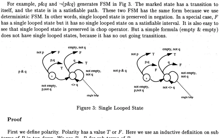
interval state.

For example,

p&q

and $\neg(p\ q)$ generates FSM in Fig 3. The marked state has

a

transition to

itself, and the state is in

a

satisfiable path. These two FSM has the

same

form because

we use

deterministic FSM. In other words, singlelooped state is preserved in negation. In

a

specialcase, $F$

has

a

single looped state but it has

no

single looped state

on a

satisfiable interval. It is also

easy

to

see

that single looped state is preserved in chop operator. But

a

simple formula (empty&empty)

does not have single looped states, becauseit has

no

out going transitions.

p&q notp&q

Figure 3: Single Looped State

Proof

First

we

define polarity. Polarityhas

a

value $T$

or

$F$. Here

we

use an

inductive definition

on

sub

terms of $P$ in top-down. We

use

$P_{s},$ $P_{t}$ for sub terms of$P$.

Initial Case $P’ \mathrm{s}$ polarity is _$T$.

Negation Case $P$ has

a

form $\neg P_{s}$. The polarity ofsub terms $P_{s}$ is negation of$P$.

Otherwise Polarity of sub terms has the

same

polarity ofparent term.

Next,

we

want to prove this. If

a

formula does not have single looped states, there

are

positive polarized empty in all positive polarized disjunction leaves, negative polarized conjunction leaves

and chop leaves. It is proved by another bottom up induction

on

ITL formula.

Initial Case If$P$ is local variable, $T$

or

$F$, it has

a

single looped state.

Initial Empty

Case

Positive polarized empty does not have single looped states. Negative

po-larized empty has

a

single looped state.

Chop Case $P$ has

a

form $P_{s}\ P_{t}$. If either $P_{s}$

or

$P_{t}$ has the

a

single looped state, $P$ has

a

single

looped state.

Negation Case $P$ has

a

form $\neg P_{s}$. If $P_{s}$ has

a

single looped state, $P$ has

a

single looped state.

Recall$F$ has

a

singleloopedstate andthe shapeof deterministic FSMis preserved innegation.

Disjunction Case $P$ has

a

form $P_{s}P_{t}$. If polarity of $P$ is positive and if either $P_{s}$

or

$P_{t}$ has

a

single looped state, $P$ has

a

single looped state. If polarity of $P$ is negative and if both $P_{s}$

Conjunction Case $P$ has

a

form $P_{s}\wedge P_{t}$. Ifpolarity of$P$ is positive and ifboth $P_{s}$ and $P_{t}$ has

a

single looped state, $P$ has

a

single looped state. If polarity of $P$ is negative and if either $P_{s}$

or

$P_{t}$ has

a

single looped state, $P$ has

a

single looped state.

These

are

easily verified by the semantics of operators and characteristics of deterministic FSM.

Roughly saying, the basic

case

shows

we

have

no

single looped states if and only if

we

have positive

emptyin it, and other induction

cases

show it is preserved in all LocalITL operators (except closure

or

next).

Assume $P$ does not have

a

single looped state in each state of the infinite satisfiable interval.

Then in all positive polarized disjunction leaves, negative polarized conjunction leaves and chop leaves, all the sub terms have positive polarized empty. This

means

$P$ is only satisfiable in

an

empty interval. It contradicts the assumption that $P$ is

satisfi..able

in

an

infinite interval. End

Proof

Evenp$(p)$

means

$p$ is true at every

even

clock period. The FSM for Even$(p)$ is

easy

as

in Fig. 4

and it does not have single looped state in the satisfiable interval. (But it has

a

single loop state

on

the unsatisfiable interval because it contains $F$ leaf) So

we

cannot express Evenp$(p)$ in Local

ITL, which is easily written in Regular Expression

or

QPTL.

$\mathrm{T}$

evenp(p)

$\mathrm{p}$

Figure 4: FSM of Evenp

The extension of the proof for including next operator is possible but not

so

easy.

It requires

careful handling of empty and next interaction. We

can

express Evenp$(p)$ for

a

fixed finite interval

using next operator, but in

case

of infinite intervals, there is

a

sub interval which is generated by

non

next restricted

way.

The sub interval has single looped state.

It is easy to show that

a

closure operator does not keep the single looped state. $\mathrm{I}\dot{\mathrm{f}}$

we

have

a

quantifier, the form of FSM changes drastically by quantifier and

we

cannot extend the proof.

Since Evenp$(p)$ is easily written with

a

closure

or a

quantifier, Even$(p)$

can

be

us.ed

as

a

counter

Appendix:

List

of

Definitions

$f\dot{i}n(P)$ $\equiv$ (T&(emptyA $P$))

$beg(P)$ $\equiv$ (($\mathrm{e}\mathrm{m}_{\mathrm{P}^{\mathrm{t}\mathrm{y}}}$ A P)&T) @P $\equiv$ $\neg \mathrm{e}\mathrm{m}\mathrm{p}\mathrm{t}\mathrm{y}\wedge \mathrm{O}^{P}$

$\mathrm{O}P$ $\equiv$

T&P

$\mathrm{O}_{S}P$ $\equiv$

S&P

$\square P$ $\equiv$ $\neg(T\ \neg P)$

$\Phi P$ $\equiv$

T&P&T

a $P$ $\equiv$ $\neg(T\ \neg P\ \tau)$

less (2) $\equiv$ OOemPty

length(2) $\equiv$ @@empty $\Phi P$ $\equiv$

P&T

$\mathrm{i}P$ $\equiv$ $\neg(\neg P\ T)$

References

[1] Rajeev Alur. The Theory of Timed

_Automat.a.

In Real-time:

_Theory.

in Practice, LNCS 600.

Springer-Verlag, 1991.

[2] R. E. Bryant. Graph-based algorithms for boolean function manipulation. IEEE Transactions

on

Computers, Vol. C-35, No. 8, pp. 667-691, August 1986.

[3] Masahiro Fujita and Shinji Kono. Synthesis of Contrllers from Interval Temporal Loigc Spec-ification. In International

_Conference

on Computer Design, October 1993.

[4] Masahiro Fujita and Shinji Kono. Synthesisof Contrllers from Interval Temporal Loigc

Spec-ification. International Workshop

on

Logic Synthesis, May 23-26, 1993.

[5] Robert Goldblatt. Logic

_of

Time and Computation, volume 7 of CSLI Lecture Notes. CSLI,

1987.

[6] M.J.C. Gordon and T.F. Melham. Introduction to the hol system. Technical report, Cambridge

University, 1994.

[7] J. E. Hopcroft and J. D. Ullman. Introduction to automata theory, language and computation.

Addison-Wesley, 1979.

[8] Shinji Kimura and Shuzou Yajima. Formal languages satifing temporal logic formula. IECE

Japan, Vol. J70-D, No. 1, pp. 117-123,

1987.

in Japanese.

[9] Shinji Kono. A Combination of Clausal and Non Clausal Temporal Logic Program. In Exe-cutable Modal and Temporal Logics, volume LNAI-897. Springer-Verlag, 1994. Lecture Notes

in Artifificial Intelligence.

[10] K.L. McMillan. “symbolic model checking: An approach to the state explosion problem”.

Technical Report CMU-CS-92-131, Carnegie Mellon University, May

1992.

[11] R. Milner. A Calculus

_of

Communicating Systems, volume 92 of Lecture Note in Computer

[12] B.C. Moszkowski. Executing temporal logic

programs.

Technical Report 55, $\mathrm{c}_{\mathrm{o}\mathrm{m}\mathrm{u}}\mathrm{p}\mathrm{t}\mathrm{e}\mathrm{r}.\mathrm{L}\mathrm{a}\mathrm{b}\mathrm{o}-$

ratory, Univ. of Cambridge,

1984.

[13] P. Wolper. Temporallogic

can

be

more

expressive. In 22nd Annual Symposium

on

Foundation