A structured pattern matrix algorithm for multichain Markov decision processes(Mathematics of Optimization : Methods and Practical Solutions)

202

A

structured pattern

matrix

algorithm for

multichain

Markov

decision

processes

宮崎大学・教育文化学部 伊喜 哲一郎 (Tetsuichiro IKI)

Faculty of Education and Culture, Miyazaki University

東京電機大学・情報環境学部 堀口 正之(Masayuki HORIGUCHI)

School of Information Environment, Tokyo Denki University

千葉大学・教育学部 蔵野 正美 (Masami KURANO)

Faculty of Education, Chiba University

Abstract

In this paper, we

are

concerned with a new algorithm for multichain finite

state Markov decisionprocesses whichfinds an average optimal policy through

the decomposition of the state space into

some

communicating classes and a

transient class. For each communicating class,

a

relatively optimal policy is

found, which is usedto find

an

optimal policy by applying the value iteration

algorithm. Using

a

pattern matrix determining the behaviour pattern of the

decision process, the decomposition of the state space is effectively done,

so

that the proposed algorithmsimplifiesthestructured

one

givenbythe excellent

Leizarowitz’s paper (Mathematicsof Operations Research, 28, 2003, 553-586).

Also, a numerical example is given to comprehend the algorithm.

Key words: multichain Markov decision processes, structured algorithm,

communicating class, transient class, value iteration.

1

Introduction and

notation

In this paper, we are concerned with the structured pattern matrix algorithm for

mul-tichain finite state Markov decision processes (MDPs) with an averagereward criterion.

The efficient algorithm for finding

an

optimal policy in average rewardMDPs have been

studied by many authors (cf. [5, 8, 11, 12, 14]). For the unichain or communicating

case, the optimal policy

can

be found by solving a single optimality equation (cf. [11]).

However, for the multichain case, the optimal policy is characterized by two equations,

called the multichain optimalityequations, which are solved, for example, by linear

pro-gramming (cf. [6, 11]) or policy iteration algorithms (cf. [7, 8]),

Recently, Leizarowitz[10] have developed the

new

algorithm for multichain average

reward MDPs, in whichtheproblem is broken into several communicating models and a

transient modeland for eachmodel, anoptimal policyis found by solving the

correspond-ing single optimality equation. The objective of this paper is to propose

a

structured

algorithm for the multichain finite state MDPs which simplify the Leizarowitz’s

sug-gestive algorithm by

use

ofpattern matrix representation of transition probabilities in

MDPs and the idea of the value iteration algorithm (cf. [5, 11]), That is, by the

203

several maximum communicating classes and a transient class and easily find the

max-imum sub-MDPs. In addition, the findingof an optimal policy is done by applying the

value iteration algorithm.

In the reminder ofthissection,

we

will define finite state MDP$\mathrm{s}$to be examined and

describe the basic results for the communicating

case.

We define

a

controlled dynamic system with

a

finite state space denoted by $S=$

$\{1,2, \ldots, N\}$

.

Associatedwith each state$\mathrm{i}\in S$is

a

non-empty finite set $A(\mathrm{i})$ ofavailable

actions. Whenthe system is instate$\mathrm{i}\in S$ and action $a\in A(\mathrm{i})$ istaken, thenthesystem

moves

to a new state $j\in S$ with probability $q_{i\mathrm{j}}(a)$ where $\sum_{j\in S}q_{ij}(a)=1$ for all $\mathrm{i}\in S$

and $a\in A(\mathrm{i})$ and the reward $r(i, a)$ is earned. The process is repeated from the

new

state $j\in S$

.

This

structure

is called a Markov decision process, denoted by

an

$\mathrm{M}\mathrm{D}\mathrm{P}$

$\Gamma=$ $(S, \mathrm{A}(\mathrm{i})$ : $\mathrm{i}\in S$

},

$Q,$$r$), where $Q=(qij(a) : \mathrm{i}, j\in S, a\in A(\mathrm{i}))$ and $r=r(\mathrm{i}, a)\in \mathrm{R}$

for all $\mathrm{i}\in S$ and $a\in A(\mathrm{i})$ and $\mathbb{R}$ is the set of all real numbers. The set of admissible

state-action pairs will be denoted by

$\mathrm{K}$$=\{(\iota, a) : i\in S, a\in A(\mathrm{i})\}$.

The samplespace isthe product space $\Omega=\mathrm{K}^{\infty}$ such that the projection $(X_{t}, \triangle_{t})$ on the

t-thfactor describes the state andaction at the $t$-thtime of the process $(t\geqq 0)$. A policy

$\pi=$ $(\pi_{0}, \pi_{1?}\ldots)$ is asequenceofconditionalprobabilitieswith$\pi t(A(xt)|x0, a0, \ldots, xt)=1$

for all histories $(x_{0}, a_{0}, \ldots, x_{t})\in \mathrm{K}^{t}S(t\geqq 0)$ where $\mathrm{K}^{0}S=S$. The set of all policies is

denoted by $\Pi$. A policy _$\pi=$ $(\pi_{0}, \pi_{1}, \ldots)$ is called randomized stationary ifa conditional

probability $\gamma=(\gamma(\cdot|i) : \mathrm{i}\in S)$ given $S$ for which $\pi(\backslash |x_{0}, a_{0}, \ldots, x_{t})=\gamma(\cdot|x_{t})$ for all $t\geqq 0$

and (Xt,$a_{0},$

$\ldots,$$x_{t}$)

$\in \mathrm{K}^{t}S$. Such a policy is simply denoted by $\gamma$. We denote by $F$ the

set of functions on $\mathrm{S}$ with $f(\mathrm{i})\in A(?.)$ for all $i\in S$. A randomized stationary policy $\gamma$ is

called stationary if there exists a function $f\in F$ such that $\gamma(\{f(\mathrm{i})\}|\mathrm{i})=1$for all $\mathrm{i}\in S$,

which is denoted simply by $f$. For each $\pi\in\Pi$, starting state $X_{0}=\mathrm{i}$, the probability

measure

$P_{\pi}(\cdot|X_{0}=\mathrm{i})$ on $\Omega$ is defined in an usual way. The problem

we are

concerned

with is the maximization of the long-run expected average reward per unit time, which

is defined by

(1.1) $\psi(\mathrm{i}, \pi)=\lim_{Tarrow}\inf_{\infty}$$\frac{1}{T}E_{\pi}(\sum_{t=0}^{T-1}r(X_{t}, \triangle_{t})|X_{0}=i)$ ,

where $E_{\pi}(\cdot|X_{0}=i)$ is the expectation w.r.t. $P_{\pi}(\cdot|X_{0}=\mathrm{i})$.

A policy $\pi^{*}\in$ II satisfying that

(1.2) $\psi(i, \pi^{*})=\sup_{\pi\in\Pi}\psi(\mathrm{i}, \pi):=\psi^{*}(\mathrm{i})$ for all

$\mathrm{i}\in S$

is called to be average optimal or simply optim al.

The structured algorithm treated with in this paper is based on a

com

municating

model

introduced

by Bather[l]. We say that the MDP $\Gamma$ is communicating if there

exists

a

randomized stationary policy $\gamma=$ $(\gamma(\cdot|\mathrm{i}) :\mathrm{i}\in S)$ satisfying that the transition

matrix$Q(\gamma)$ induced by$\gamma$ defines a irreducibleMarkov chain where

$Q(\gamma)=(q_{ij}(\gamma))$ with

Lemma 1.1. For the communicating MDP $\Gamma$, there exists a constant g and a vector

v $=$ $(v_{i}$: i $\in S)$ such that

(1.3) $v_{i}+g= \max_{a\in A\langle i)}\{r(i, a)+\sum_{j\in S}q_{\iota j}(a)v_{j}\}(\mathrm{i}\in S)$

and any stationary policy$f^{*}$ such that $f^{*}$ attains the maximum

of

(1.3) is optimal with

$g=\psi(\mathrm{i}_{7}f’)$ $= \sup_{\pi\in\Pi}\tau\ell(\mathrm{i}, \pi)$

for

all $\mathrm{i}\in S$.

We note that the algorithm for finding anoptimal policy in Lemma 1.1

are

given as

the value iteration

or

policy iteration algorithms (cf. [11]).

In Section 2, the methods ofclassifying the set of states by use of the corresponding

pattern matrices is proposed, whichisused to find

a

optimal policy bythevalue iteration

algorithm in Section 3. In Section 4,

a

numerical example is given to comprehend

our

structured algorithm.

2

Pattern

matrices

and

state classification

In this section,

we

define a pattern matrix for the transition matrix of the MDPs which

is used to classify the state space and find the maximum sub-MDPs.

For a non-empty sub set $D$ of $S$, if, for each $\mathrm{i}\in D$, there exists a non-empty subset

$\overline{A}(i)\subset \mathrm{A}(\mathrm{i})$ with_{$\sum_{j\in D}q_{ij}(a)=1$} for all$a\in\overline{A}(\mathrm{i})$,

we can

consider thesub-MDPwiththe

restricted state space $D$ and available action space $\overline{A}(i)$ for $\mathrm{i}\in D$, which is denoted by

$\overline{\Gamma}=$ _{$(D, \{\overline{A}(\mathrm{i}) : \mathrm{i}\in D\}, Q_{D}, r_{D})$}where _{$Q_{D}$} and

$r_{D}$ are restriction of $Q$ and $r$ on

{

$(i, a)$ : $\mathrm{i}\in D$,$a\in\overline{A}(\mathrm{i})\}$. Forany sub-MDP$\overline{\Gamma}=(D, \{\overline{A}(\mathrm{i}) :\mathrm{i}\in D\}, Q_{D}, r_{D})$, anon-emptysubset

$\overline{D}$ of

$D$ is a communicating class in$\overline{\Gamma}$

if$\overline{D}$

is closed, that is, $\sum_{g\in\overline{D}}qij(a)=1$ for all$\mathrm{i}\in\overline{D}$

and $a\in\overline{A}(\mathrm{i})$ and the sub-MDP $(\overline{D}, \{\overline{A}(\mathrm{i}) :\mathrm{i}\in\overline{D}\}, \mathrm{Q}\mathrm{D}, r_{\overline{D}})$ is communicating Also,

$\overline{D}$

is maximum communicating class if it is not strictly containedin any communicating

class.

For any positive integer 1, let $\mathbb{C}^{f}$ and $\mathbb{C}^{l\mathrm{x}l}$ be the sets of $l$-dimensional

row

vectors

and $l\mathrm{x}$ $l$ matrices with

{0,

1}-valued

elements, respectively. The

sum

$(+)$ and product

($\cdot$) operators among elements in

$\mathbb{C}^{l}$ and $\mathbb{C}^{l\mathrm{x}l}$

is defined by $a+b= \max\{a, b\}$ and $a\cdot$ $b=$

$\min\{a, b\}$ for $a$,$b\in\{0,1\}$.

For each $\mathrm{i}\in S$ and $a\in A$, we define _{$m_{i}(a)=(m_{i1}(a), m_{i2}(a),$}

$\ldots$ ,$m_{iN}(a))\in \mathbb{C}^{N}$ by

$(2.1\rangle$ $m_{ij}(a)=\{$1 if

$q_{i\mathrm{i}}(a)>0$,

0

if $q_{ij}(a)=0$,

$(j\in S)$_.

For a sub-MDP $\overline{\Gamma}=$ _{$(D\rangle\{\overline{A}(\mathrm{i}) : i\in D\})Q_{D)}r_{D})$} with $D=$

{

$\mathrm{i}_{1}$,i2,

$\ldots$ ,

$\mathrm{i}_{l}$

},

we

put

$m_{i}(\overline{\Gamma})=(m_{ii_{1}}(\overline{\Gamma}), m_{ii_{2}}(\overline{\Gamma})$,

. .. ,$m_{ii_{l}}( \overline{\Gamma}))=\sum_{a\in\overline{A}(i)}m_{i}(a|\overline{\Gamma})(\mathrm{i}\in D)$, where$m_{i}(a|\overline{\Gamma})$ $=(m_{ii_{1}}(a), m_{ii_{2}}(a),$$\ldots$ ,$m_{ii_{l}}(a))(x$ $\in$ $D$, $a\in\overline{A}(\mathrm{i}))$

.

Using $m_{i}(\overline{\Gamma})(\mathrm{i}\in D)$,

we

define apattern matrix $M(\overline{\Gamma})$ for the sub-MDP

205

$\overline{\Gamma}$by

(2.2) $M(\overline{\Gamma})=(\begin{array}{l}m_{i_{\mathrm{l}}}(\overline{\Gamma})\vdots m_{i_{f}}(\overline{\Gamma})\end{array})$ $\in \mathbb{C}^{l\mathrm{x}l}$.

We note that for $i$,$j\in D$, $m_{ij}(\overline{\Gamma})=1$

means

that there exists $a\in\overline{A}(\mathrm{i})$ with $q_{ij}(a)>0$.

The pattern matrix defined above is called a communication matrix (cf. [10]).

How-ever,since $M(\overline{\Gamma})$ determines the behaviour pattern of thesub-M DP

$\overline{\Gamma}$

,

we

callit apattern

matrix in this paper. For the pattern matrix $M(\overline{\Gamma})$,

we

define $\overline{M}(\overline{\Gamma})\in \mathbb{C}^{ll})\langle$ by

(2.3) $\overline{M}(\overline{\Gamma})=\sum_{k=1}^{N}M(\overline{\Gamma})^{k}$.

Then,

we

have the following.

Lemma 2.1. For a non-empty subset$\overline{D}$

of

$D$, $\overline{D}$

is a communicating class

_if

and only

if,

_for

each $\mathrm{i}\in\overline{D}$,

$\overline{m}_{ij}(\overline{\Gamma})=\{$

1if

$j\in\overline{D}$,

0if

$j\not\in\overline{D}$,

where $\overline{m}_{ij}(\overline{\Gamma})$ is the $(\mathrm{i},j)$ element $of\overline{M}(\overline{\Gamma})$ and $\overline{M}(\overline{\Gamma})=(\overline{m}_{ij}(\overline{\Gamma}))$.

Proof.

See Appendix.1

By reordering the states in $D$, $\overline{M}(\overline{\Gamma})$

can

be transformed to the standard form:

(2.4) $\overline{M}(\overline{\Gamma})=(\begin{array}{lll}E_{1} ---- \overline{\overline{E}}_{2}--\backslash )1 ---- 0.---,-.-.--.-|---0_{\downarrow\overline{E}_{d_{\underline{t}}^{1}}^{\iota_{!}}}\overline{R}\prime\overline{\overline{K}}\vee---\neg \end{array})$ $(d\geqq 1)$,

where $E_{j}$ is a square matrix whose elements are all 1 $(1\leqq j\leqq d)$ and $[RK]$ does not

include a sub-matrix having the above form.

For any sets $U,$ $V$, if $U\cap V=\emptyset$,

we

write the union $U\cup V$ by $U+V$.

Here,

we

get the classification ofthe state space.

Theorem 2.1. For a sub-MDP $\overline{\Gamma}=$ _{$(D, \{\overline{A}(\mathrm{i}) : i\in D\})Q_{D)}r_{D})$}, the state space $D$ is

classified

as

follows;

(2.5) $D=U_{1}+U_{2}+\cdots+U_{d}+L(d\geqq 1))$

where $U_{j}$ is a comrmrnicating class

for

$\overline{\Gamma}(1\leqq j\leqq d)$ and

$L$ is not closed.

Proof.

See $\mathrm{A}\mathrm{p}\mathrm{p}\mathrm{e}\mathrm{n}\mathrm{d}\mathrm{i}\mathrm{x}_{\mathrm{I}}$

.

The algorithm of obtaining the state-decomposition (2.5) through (2.4) by

use

of the

pattern matrix willbe called Algorithm A.

When the not-closedclass $L$ in (2.5) is non-empty,

we

go

on

with the state

classifica-tion of $L$ by finding the maximum sub-MDP. The basic idea of the following algorithm

Algorithm B:

1. Set $K_{1}=L$.

2. Suppose that $\{K_{i} : 1\leqq \mathrm{i}\leqq n\}$ with $K_{1}\neq\supset K_{2}\neq\supset\ldots\neq\supset K_{n}(K_{n}\neq\emptyset)$ is given.

Then, set $V=S-K_{n}$ and each $\mathrm{i}\in K_{n}$, set $A_{1}(i)=A(i)-T(\mathrm{i})$, where $T(i)=$

$\{a\in A(\mathrm{i})|\sum_{j\in V}m_{ij}(a)=1\}$.

Set

$K_{n+1}=\{\mathrm{i}\in K_{n}|A_{1}(\mathrm{i})\neq\emptyset\}$.

3.

The following three

cases

happen:

Case 1: $K_{n+1}\neq\emptyset$ and $K_{n}\supset K_{n\dagger 1}\neq$.

For this case, put $n=n+1$ and go to Step 2 with $\{K_{i} : 1\leqq \mathrm{i}\leqq n +1\}$

.

Case 2: $K_{n+1}=K_{n}$.

For this case, set $\overline{D}:=K_{n+1}$. Then, $\overline{\Gamma}=\{\overline{D}, \{A_{1}(\mathrm{i}) : \mathrm{i}\in\overline{D}\}, Q_{\overline{D}}, r_{\overline{D}}\}$ is $\mathrm{a}$

maximum sub-MDP in $L$

.

Apply Algorithm A for this sub-MDP

$\overline{\Gamma}$

.

Case 3: $K_{n+1}=\emptyset$. Step the algorithm.

For this case, the set $L$ does not include any sub-MDP and it holds that

(2.6) $\max_{i\in L,\pi\in\Pi}P_{\pi}(X_{n}\in L|X_{0}=\mathrm{i})<1$.

Starting with the MDP $\Gamma=$ $(S, \{A(\mathrm{i}) : \mathrm{i}\in S\}, Q, r)$ given firstly, we apply Algorithm

A and $\mathrm{B}$ iteratively, so that

we

get the following.

Theorem 2.2. Let $\Gamma=$ $(S, \{A(\mathrm{i}) : \mathrm{i}\in S\}, Q, r)$ be the

fixed

$MDP$. Then, there exists $a$

sequence

_of

sub-MDPs

$\Gamma_{k}=$ $(S_{k}, \{A_{k}(\mathrm{i}) : \mathrm{i}\in S_{k}\}, Q_{S_{k}}, r_{S_{k}})(k=0, 1, \ldots, n^{*})$

satisfying the following $(\mathrm{i})-(\mathrm{i}\mathrm{i})$.

(i) $S_{0}=S\supset S_{1}\neq\neq..\neq\supset.\supset g_{n^{*}}$

(i) The state space $S$ is decomposed to:

(2.7) $S=U_{0}+U_{1}+\cdots+U_{n}*+L$,

where

(2.8) $U_{k}=U_{k1}+U_{k2}+\cdots+U_{kl_{k}}(0\leqq k\leqq n^{*})$,

$U_{kj}(1\leqq j\leqq l_{k})$ is a mctzirrvum communicating class $(m.c.c.)$

for

the sub-MDP

$\Gamma_{k_{1}}$ and $L$ is

a

transient class, that is,

for

any $\mathrm{i}\in L$ and $a\in A(\mathrm{i})_{f}$ there exists

an

integer$n\geqq 1$ such that

(2.9) $\max P_{\pi}(X_{n}\in L|X_{0}=\mathrm{i})<1$.

207

Applying Lemma 1.1 to each communicating sub-MDP $\Gamma_{kj}=(U_{kj}$,

{

$A_{k}(\mathrm{i})$ : $\mathrm{i}\in$

$U_{kj}\}$,$Q_{U_{kj}}$,$r_{U_{kj}})$,

we

get an optimal stationary policy $f_{kj}$ and

an

optimal average reward

$g_{kj}$ for

$\mathrm{s}\mathrm{u}\mathrm{b}arrow \mathrm{M}$ DP $\Gamma_{kj)}$ called relatively $0.\mathrm{p}$. and relatively $\mathrm{a}.\mathrm{r}.$, respectively, which is

summarized in Table 2.1.

Table 2.1: Relatively $0.\mathrm{p}$. and $\mathrm{a}.\mathrm{r}$.

We note that a stationary policy $f_{0j}$ is absolutely optimal on $U_{0j}(1\leqq j\leqq l_{0})$ because

optimization is done in the MDP $\Gamma$.

3

Algorithm for

obtaining

an

optimal

policy

In this section,

we

give

a

value iterative algorithm based

on

datain Table 2.1 to find

an

(absolutely) optimal policy for the $\mathrm{M}\mathrm{D}\mathrm{P}\Gamma$.

Let $K_{L}:=$

{

$(\mathrm{i}$,$a$)$|\mathrm{i}\in L$ and $a\in A(\mathrm{i})$

}

and $B(L)=\{v|v : Larrow \mathbb{R}\}$. For any function $d$ on $K_{L}$, the map $T_{d}$ : $B(L)arrow B(L)$ will be defined

as

(3.1) $T_{d}v( \mathrm{i})=\max_{a\in A(i)}\{d(i, a)+\sum_{j\in L}q_{ij}(a)v(j)\}(\mathrm{i}\in L)$.

We need the following lemma to treat with thetransient class L in Theorem 2.2.

Lemma 3.1. (of. f3]) Thefollowing holds:

(i) The map $T_{d}$ is an $n$-step contraction, that is, $||T_{d}^{n}v-T_{d}^{n}v’||\leqq\beta||v-v’||$

for

some

$0<\beta<1$ ancl$v$,$v’\in \mathrm{B}(\mathrm{L})$, where $n$ is

as

that in (2.9).

(ii) $T_{d}$ is monotone, that is,

if

$v\leqq v’$,$T_{d}v\leqq T_{d}v’$.

(Hi) Denote by$v\{d\}$ a unique

fixed

point

of

$T_{d}$. Then,

if

$d\leqq d’$,$v\{d\}\leqq v\{d’\}$.

Proof

See $\mathrm{A}\mathrm{p}\mathrm{p}\mathrm{e}\mathrm{n}\mathrm{d}\mathrm{i}\mathrm{x}_{1}$.

Let $\mathcal{K}=\{(s,j)|0\leqq s\leqq n^{*}, 1\leqq j\leqq l_{s}\}$ where $n^{*}$ and $l_{s}$

are

given in Theorem 2.2.

For $D\subset S$, let $q_{i}(D|a):= \sum_{j\in D}q_{ij}(a)$. In the ensuring discussion,

we

give the value

iteration algorithm, called Algorithm $\mathrm{C}$, for finding

an

optimal policy starting with

data in Table 2.1.

Algorithm C.

1. Set $n=1$,$g_{sj}(1)=g_{sj}$ for $(s,j)\in \mathcal{K}$ and $g_{i}(1)=v\{d_{1}\}(\mathrm{i})$ for $\mathrm{i}\in L$,

2. Suppose that $\{g_{sj}(n) : (s, j)\in \mathcal{K}\}$ and $\{g_{i}(n) : \mathrm{i}\in L\}$

are

given $(n\geqq 1)$.

Let for $\mathrm{i}\in S-L$,

(3.2) $g_{i}= \max_{a\in A(i)}\{d_{n}(\mathrm{i}, a)+\sum_{j\in L}q_{ij}(a)g_{j}(n)\}$,

where $d_{n}( \mathrm{i}_{7}a)=\sum_{(s,j\}\in \mathcal{K}}q_{i}(U_{sj}|a)g_{sj}(n)$.

Let $g_{sj}(n+1)= \max_{i\in U_{sj}}g_{i}$ and $g_{i}(n +1)=v\{d_{n}\}(\mathrm{i})$ for $\mathrm{i}\in L$.

3. Let $n=n+1$ and go to Step 2.

Concerning with Algorithm $\mathrm{C}$,

we

have the following.

Lemma 3.2. In Algorithm C,

we

have:

(i) It holds that

(3.3) $gsj(n+1)\geqq g_{sj}(n)$

for

$(s, j)\in \mathcal{K}$, and

(3.4) $g_{i}(n +1)\geqq g_{i}(n)$

for

$i\in L$.

(ii) The Algorithm $\mathrm{C}$ converges, $\mathrm{i}.e.$, rnhen _$narrow$ oo $g_{sj}(n)$ $arrow\overline{g}_{sj}$

for

$(s,j)\in \mathcal{K}$ and

$g_{i}(n)arrow\overline{g}_{i}$

for

$\mathrm{i}\in L$.

Proof

See $\mathrm{A}\mathrm{p}\mathrm{p}\mathrm{e}\mathrm{n}\mathrm{d}\mathrm{i}\mathrm{x}.\iota$

For $\overline{g}_{sj}$ and $\overline{g}_{i}$ in Lemma 3.2,

we

have the following.

(3.5) $\overline{g}_{sj}=\max_{a\in A(\mathrm{z})}\{d(\mathrm{i}, a)+\sum_{j\in L}q_{i_{J}}(a)\overline{g}_{j}\}$ for

$\mathrm{i}\in U_{sj}$ and $(s,j)\in \mathcal{K}$,

and

(3.6) $\overline{g}_{i}=\max_{a\in A(i)}\{d(\mathrm{i}, a)+\sum_{j\in L}q_{ij}(a)\overline{g}_{j}\}$ for

$\mathrm{i}\in L$,

where $d( \mathrm{i}, a)=\sum_{(s,j)\in \mathcal{K}}q_{i}(U_{Sji}|a)\overline{g}_{sj}$ .

Let $f^{*}$ be any stationary policy such that

(3.7) $f^{*}(\mathrm{i})=\{$

$f_{\mathrm{o}j}(i)$ for $i\in U_{0\mathrm{j}}(1\leqq j\leqq l_{0})$

any maximizer in (3.5) and (3.6) for $i\in S_{1}$.

Theorem 3.1. The stationary policy $f^{*}$ is optimal and

$\psi(\mathrm{i}, f_{/}^{*})=\overline{g}_{sj}$

for

$\mathrm{i}\in U_{sj}$, $(s, j)\in \mathcal{K}$, and $\psi(\mathrm{i}, f^{*})=\overline{g}_{i}$

for

$\mathrm{i}\in L$.

Proof

See $\mathrm{A}\mathrm{p}\mathrm{p}\mathrm{e}\mathrm{n}\mathrm{d}\mathrm{i}\mathrm{x}_{\mathrm{I}}$.

The dynamic programming (DP) algorithm associated with MDPs has to compute

a

suitablydefinedvaluefunction onthe state space, which gives rise to the difficulties called

$‘(\mathrm{c}\mathrm{u}\mathrm{r}\mathrm{s}\mathrm{e}$ofdimensionality” whenapplyingthe DP algorithm to theproblem involvingvery

large state space (cf. [2, 4]). In the structured algorithm developed in this section, the

state spacemay be partitioned into several classes ofa small number of states. This may

be

a

wayto

overcome

thedifficulties mentioned above. The availability of

our

algorithm

depends deeply

on

the structure of the model.

So

that it may have the possibility of

reducingthe amountofcomputationandthe number ofstepsrequired inthe computation

2Ofl

4

A

numerical

example

Inthissection, wegive

a

numerical exampleto comprehend

our

structured algorithm for

the multichain

case.

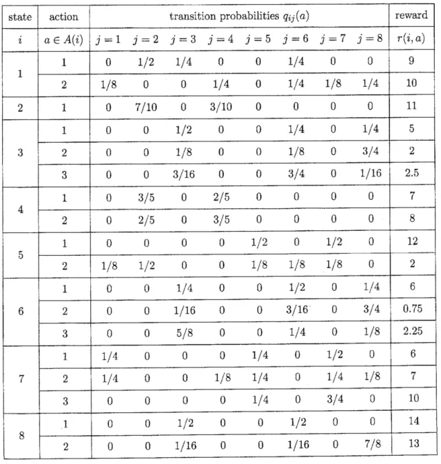
Let

us

find theoptimality policy for the eight-state MDP with$S=\{1,2,3,4,5,6,7,8\}$

and $A(1)=\{1,2\}$,$A(2)=\{1\}$,$A(3)=\{1,2,3\}$,$A(4)=\{1,2\}$,$A(5)=\{1,2\}$,$A(6)=$

$\{1,2,3\}$,$A(7)=\{1,2\}$ and $A(8)=\{1,2,3\}$, whose transition probability matrix and

rewards

are

given in Table

4.1.

Table 4.1: A numerical example

$M=(m_{ij})$ in (2.2) and $\overline{M}=(\overline{m}_{ij})$ in (2.3)

are

easily computed, which

are

shown

as

follows.

123 4 5 6 7 $\mathrm{s}$ 123 4 5 6 7 8

M $=$

86543271

$\ovalbox{\tt\small REJECT}$

0000011100001111000011110000111100000011

0OOIIIII

0000011100011111

$\ovalbox{\tt\small REJECT}$ ,

$\overline{M}=$

37654821

$\ovalbox{\tt\small REJECT}$

00000111

00011111

00111111

0001111100000111

00111111

0000011100111111

$\ovalbox{\tt\small REJECT}$

.

By reorderingofthe states, $\overline{M}$

is transformed

as

follows (abusing the notation).

3 6 s 2 4 1 5 7

$\overline{M}=$

43728651

$\ovalbox{\tt\small REJECT}-.---,\ulcorner^{---\neg---}\downarrow---arrow"‘---.\ovalbox{\tt\small REJECT} 11111_{\iota}^{\mathfrak{l}}11_{\iota}^{t}|011_{j}^{1}1111111111111111\tilde{1}\overline{1}\overline{1}\overline{1}1\overline{1}\overline{1}\overline{1}0^{\mathrm{I}}111_{1}^{1}0\mathfrak{l}11\mathrm{i}.11$,

Observing the above, we have

$S=U_{01}+U_{02}+L$,

where $U_{01}=\{3_{7}6, 8\}\rangle U_{02}=\{2,4\}$, $L=\{1,5,7\}$.

Now,

we

apply Algorithm $\mathrm{B}$ to $L=\{1, 5, 7\}$. For $n=1$,

we

get the following:

$K_{1}=L=\{1,5,7\}$,$V=S-K_{1}=\{2,3,4,6_{2}8\}$,$T(1)=\{1,2\}$,

$T(5)=\{2\}$,$T(7)=\{2\}$,$A_{1}(1)=\emptyset$,_{$A_{1}(5)=\{1\}$},$A_{1}(7)=\{1, 3\}$.

So that $K_{2}=\{5,7\}$. Thus,

we

have found the maximum sub-MDP:

$\Gamma_{1}=(S_{1}=\{5,7\})\{A_{1}(\mathrm{i}) : \mathrm{i}\in S_{1}\}$,$Q_{S_{1}}$,

$r_{S_{1}}$$)$.

Applying Algorithm A to Fi,

we

find that $\Gamma_{1}$ is communicating. In the end, the

decomposition of$S$ in (2.7) is shown

as:

$S=U_{01}+U_{02}+U_{11}+L$ with _$L=\{1\}$ and data

211

Table 4.2; _Relatively $0.\mathrm{p}$. and $\mathrm{a}.\mathrm{r}$. for a numerical example

Here, to find

an

optimal policy, we apply Algorithm $\mathrm{C}$ to Table 4.2, Since, $/\mathrm{o}\mathrm{i}$ and

/02

are

absolutely optimal, it holdsthat $g_{01}$$(n)=11.333$ and$g_{02}(n)=9.714$ for all$n$

$\geqq 1$

and $f^{*}(3)=f^{*}(6)=f^{*}(8)=2$,$f^{*}(2)=1$,$f^{*}(4)=2$. For $n=1$,$g_{11}(1)=$

10.667

and

$g_{1}(1)=v\{d_{1}\}(1)=$ lC1776 is obtained

as

a unique solution of the following equation

from Lemma 3.1:

$g_{1}(1)= \max\{\frac{1}{2}g_{01}(1)+\frac{1}{2}g_{02}(1)$, $\frac{1}{2}g_{01}(1)+\frac{1}{4}g_{02}(1)+\frac{1}{8}g_{11}(1)+\frac{1}{8}g_{1}(1)\}$

$= \max\{10.524,9.429$$+ \frac{1}{8}g_{1}(1)\}$ .

By $(3,2)$,

we

get that $g_{5}=$

10.667

and $g_{7}=10,694$

.

So, $g_{11}(2)= \max\{g_{5}, g_{7}\}=10.694$

and $g_{1}(2)=$

10.776.

Similarly,

we

get that $g_{11}(3)=10.794$,$g_{1}(3)=10.779$ and $g_{11}(4)=$

10.731,$g_{1}(4)=$

10.782.

We proceed withrepeating thestep $n$until $|g_{11}(n)-g_{11}(n+1)|<$

$\epsilon=10^{-4}$ and _{$|g_{1}(n)-g_{1}(n+1)|<\epsilon$} simultaneously. Then, we find that $\overline{g}_{11}\cong 10.794$

and $\overline{g}_{1}\cong$

10.794.

From Theorem 3.1,

we

get optimal policy in other states

as

$f^{*}(5)=$

$1$,$f^{*}(7)=3$,$f^{*}(1)=2$ and the optimal value $\psi^{*}(3)=\psi^{*}(6)=\psi^{*}(8)=11.333$ $\psi^{*}(2)=$

$\psi^{*}(4)=$ 9.714,$\psi^{*}(5)=\psi^{*}(7)\cong 10,794,$$\psi^{*}(1)\cong 1$(1794

Appendix

ProofofLemma 2.1

Let $\overline{D}$ be

a

communicating class. By the definition,

$\overline{D}$ is closed, so that for $\mathrm{i}\in\overline{D}$ and

$j\not\in\overline{D}$, $P_{\pi}(X_{t}=j|X_{0}=\mathrm{i})=0$ for all $t\geqq 1$ and $\pi\in\Pi$, which

means

$\overline{m}_{ij}(\overline{\Gamma})=0$. Also,

there exists a randomized stationary policy $\gamma$ such that

$Q_{\overline{D}}(\gamma)$ determines

a

irreducible

Markov chain, so that for $\mathrm{i},j\in\overline{D}$, _{$P_{\gamma}(X_{t}=j|X_{0}=\mathrm{i})>0$} for

some

$t(0\leqq t\leqq N)$.

Thus, $\overline{m}_{ij}(\overline{\Gamma})=1$ follows for $\mathrm{i},j\in\overline{D}$. The proof ofthe “if” part follows

$\mathrm{o}\mathrm{b}\mathrm{v}\mathrm{i}\mathrm{o}\mathrm{u}\mathrm{s}1\mathrm{y}_{1}$.

Proof ofTheorem 2.1

Let $U_{j}$ and $L$ be the sets of states corresponding to $E_{j}$ and $K$ in (2.4), respectively,

$(1 \leqq j\leqq d)$_{. Then, from Lemma 2.1,} $U_{j}$ is

a

communicating class. If $L$ is closed,

$\overline{\overline{\Gamma}}=$

$(L, \{\overline{A}(\mathrm{i}) : \mathrm{i}\in L, Q_{L}, r_{L})\}$ is a sub-MDP. Applying the above discussion,

we

get$\overline{M}(\overline{\overline{\Gamma}})$

is

rewritten into a matrixwhich has the

same

structure

as

(2.4), which is

a contradiction..

Proof ofLemma 3.1

By (2.9), (i) clearly holds (cf. [3]). Also, (ii) follows from the definition. Let $d\leqq d’$.

.

_{Then, we have that}

This completes the proofof (iii)_.1

Proof of Lemma 3.2

Since $Usj$ is a communicating class, by the definition for each $\mathrm{i}\in U_{sj}$, there exists

$a\in A(\mathrm{i})$ such that $q_{i}(U_{sj}|a)=1$, which implies from (3.2) that $g_{i}\geqq g_{sj}(n)$. So, we get $g_{sj}(n+1)\geqq g_{sj}(n)$. Also, Lemma

3.1

(Hi), from $d_{n}\geqq d_{n-1}$ it follows that $g_{i}(n+1)=$

$v\{d_{n}\}(\mathrm{i})\geqq v\{d_{n-1}\}(\mathrm{i})=g_{i}(n)$ for $\mathrm{i}\in L$. Since $\{g_{sj}(n)\}$ and $\{g_{i}(n)\}$

are

bounded, (ii)

follows from (i). 1

Proofof Theorem 3.1

For any stationary policy $f$, let denote by $Q(f)$ the corresponding transition matrix.

The decomposition of the state space $S$ w.r.t. $Q(f)$ will be denoted by

$S=O_{1}+\cdots+O_{l}+L’$,

where $O_{i}(i=1,2, \ldots, l)$ is

an

ergodic class and $L’$ is a transient class (cf. [9]). For each

$O_{k}$, since $L$ is a transient class it is impossible that $O_{k}\subset L$. Thus, recalling that each

$Usj$ is a maximum communicating class, $O_{k}\subseteq U_{sj}$ for

some

$(s,j)\in \mathcal{K}$, which implies $\psi(\mathrm{i}, f)\leqq\overline{g}_{sj}$ for $\mathrm{i}\in O_{k}$. Also, by (3.5)-(3.6)

$)$

$\psi(i, f)\leqq\psi(\mathrm{i}, f^{*})$for $\mathrm{i}\in L’$. Theotherhalf

part of theorem holds obviously.i

References

[1] John Bather. Optimal decision procedures for finite Markov chains. II.

Communi-cating systems. Advances in AppL Probability, 5:521-540,

1973.

[2] Richard Bellman. Dynamic programming. Princeton Univeristy Press Princeton,

N. J.,

1957.

[3] Eric V. Denardo. Contractionmappings in the theory underlying dynamic

program-ming. SIAMRev., 9:165-177,

1967.

[4] Eric V. Denardo. Dynamic programming: models and applications, Prentice-Hall,

Inc., Englewood Cliffs, N. $\mathrm{J}_{\}}$

.1982.

[5] A. Federgruen and P. J. Schweitzer. Discounted and undiscounted value-iteration

in Markov decision problems: a survey. In Dynamic programming and its

applica-tions (Proc. Conf.,. Univ. British Columbia, Vancouver, B. C., 1977), pages 23-52,

Academ ic Press, New York,

1978.

[6] A. Hordijk and L. C. M. Kallenberg. Linear programming and Markov decision

chains. Management Sci., 25(4):352-362, 1979/80.

[7] Arie Hordijk and Martin L. Puterman. On the convergence of policy iteration in

finitestateundiscounted Markovdecision processes: theunichain

case.

Math, _Oper.

213

[8] Ronald A. Howard. Dynamic programming and Markov processes. The Technology

Press ofM.I.T., Cambridge, Mass., 1960.

[9] John

G.

Kemeny andJ. LaurieSnell. Finite Markov chains. The University Series in

Undergraduate Mathematics. D. Van Nostrand Co., Inc., Princeton,

N.J.-Toronto-London-New York, 1960.

[10] Arie Leizarowitz. An algorithm to identify and compute average optimal policies in

multichainMarkov decision processes. Math. Oper. Res., 28(3):553-586, 2003.

[11] Martin L. Puterman. Markov decision processes: discrete stochastic dynamic

pro-grarnming. John Wiley

&

Sons Inc., New York, 1994. A Wiley-Interscience

Publi-edition,

[12] Paul J. Schweitzer. Iterative solution of the functional equations of undiscounted

Markov renewal programming. J. Math. Anal Appl, 34:495-501, 1971.

[13] E. Seneta. Nonnegaiive matrices and Markov chains. Springer Series in Statistics.

Springer-Verlag, New York, second edition,

1981.

[14] D. J. White. Dynamic programming, Markov chains, and the method of successive