68
Automated
Competitive
Analysis of
Online
Problems
オンライン問題の競合比解析の自動化について
Shingo Masanishi*
Takashi
Horiyama*Kazuo
Iwalnar
正西申悟
堀山貴史
岩間一雄
{masanisi
,
$\mathrm{h}\mathrm{o}\mathrm{r}\mathrm{i}\mathrm{y}\mathrm{a}\mathrm{m}\mathrm{a}_{*}$iwama}Qlab2.
kuis.kyot0-u.
$\mathrm{a}\mathrm{c}$.
jp
Abstract
An online
knapsack
problem
is
an
online
problem
where
an
online
player
receives
a
sequence
of
items
one
by
one
and
on
every
arrival
of
an
item
he must decide whether he
takes
it
or
not. In
$*1\mathrm{J}1$exchangeable
online knapsack
problem
(EOK),
the player has two
(or more)
knapsacks of size 1. alld he is allowed
10
exchange
(and
also
discard)
items in his knapsacks. It is known that the
competitive
ratio of this
$\mathrm{p}\iota 01$)
$\downarrow \mathrm{e}\pi\iota$has
an
upper bound
1.3333
and
a
lower bound
1.2808
when the number of knapsack
$k$
.
is
2.
Unfortunately,
the tight bound is not known. The
di
題
culty
for
obtaining those bounds is mainly caused
by
a
large
number
of
possible
cases
to
be considered in their proofs. In this paper,
we
propose
a
$\mathrm{c}\mathrm{o}\mathrm{m}$puter
aided
analysis
on
the
competitive
ratios of
online
problems,
and
show
proofs of the upper
bounds 1.3660
and
1.333
for 2-bin
EOK.
These results do not only give
an
another proof of the known bound, but also give
a
basis for the
tight
bound.
An online
knapsack
problem
is
an
online problem
where
an
online player
$\mathrm{r}\mathrm{e}\mathrm{c}.\mathrm{e}\mathrm{j}\mathrm{v}\mathrm{a}\mathrm{e}^{\neg}$a
$\mathrm{a}\mathrm{e}\mathrm{q}\iota \mathrm{l}\mathrm{e}\mathrm{u}\mathrm{c}.\mathrm{e}$
or
$\mathrm{i}\iota \mathrm{e}1’ 1\mathrm{S}$one
by
one
and
on
every
arrival
of
an
item
he
$\mathrm{m}$ust decide whether he
takes
it
01
not.
$\ln$
*1J1
$\rho_{-}\alpha.\mathrm{c}.1_{1\aleph 11}\mathrm{g}\mathrm{e}\mathrm{a}\mathrm{t}$)
$1\mathrm{t}^{\backslash }$online knapsack
$\mathrm{p}_{10])}.1\mathrm{e}\mathrm{m}$(EOK),
the player has two
(or
$\mathrm{n}\iota \mathrm{o}\mathrm{r}\mathrm{e}$
)
$\mathrm{k}\mathrm{n}\mathrm{a}\mathrm{p}"\backslash$of
$\mathrm{s}\mathrm{i}\mathrm{z}\iota$.
1. alld hc is allowed
$(01$
exchange
(and
also
discard)
items in his knapsacks. It is known that the
competitive
ratio
or
this
$\mathrm{p}\iota 01$)
$\downarrow \mathrm{e}\pi\iota$llas
$\mathrm{m}$upper bound
1.3333
and
a
lower bound
1.2808
when the number of knapsack
$k$
is
2.
$(j11\mathrm{f}\mathrm{o}\mathrm{r}\mathrm{t}\mathrm{u}11\dot{\epsilon}1\mathrm{t}\mathrm{t}^{\backslash }1\iota’$,
the tight bound is not known. The
di
題
culty
for
obtaining those bounds is
$\mathrm{m}$ainly caused
by
$n$
large
number
of
possible
cases
to
be considered in their proofs.
$\ln$
this paper,
we
$\mathrm{P}^{1\mathrm{O}}\cdot \mathrm{p}\mathrm{o}\mathrm{a}^{\neg}\mathrm{e}$a
$\mathrm{c}\mathrm{o}\mathrm{m}$puter
aided
analysis
on
the
competitive
ratios of
online
problems,
and
show
$\mathrm{p}_{1}\cdot \mathrm{o}\mathrm{o}\mathrm{f}\mathrm{s}$of
the upper
bounds .3660
alld
1.333
for 2-bin
EOK.
These results do not only give
an
another proof of the
$\mathrm{h}_{1}\mathrm{o}\mathrm{w}\mathrm{n}$b0ll’1d, but also
$\mathrm{g}\mathrm{i}\mathrm{v}\epsilon^{1}$
a
basis for the
tight
bound.
Keywords:
Online
problems,
Online
algorithms,
Com
petitive ratio,
Knapsack
problems.
1
Introduction
An
online
$p;.oblen\iota$
gives
us a
sequence of
requests
and
asks to
respond
$\mathrm{i}$mmediately
to
each
request
without
knowing future information. Online
problems
are a
natural
topic
of interest in
many
disciplines
such
as
$\mathrm{C}^{\cdot}\mathrm{O}\mathrm{I}\mathrm{U}-$puter
science,
economics
and
operations research. Many applications
are
essentially
online,
where
illllJle(litne
decisions
are
required
in
a
real time. Paging in
a
virtual
memory
system is perhaps
tlle most studied of
$\mathrm{s}n$(41
computational problems.
Routing in communication
network
is
another
well-known
application
$[1, 2]$
.
$\mathrm{A}_{1}$al-goritlrrn
which solves
an
online
problem
is
called
an
online algorithm. On the other
$\mathrm{h}$and,
an
offline
$alq$
orithm
is
allowed
to respond to each request after receiving
all the
requests.
In other
words,
an
offline algorithm
knows the
future, while
an
online
algorithm
does
not.
The
most famous way
to
measure
the
e
題
ciency
of
online
algorithm
$\mathrm{s}$is
a
competitive
ratio,
which
is
the ratio
of the
cost
of
an
online
algorithm to that of tlle
offline
algorithm.
A
good
online
algorithm
makes
a
cornpetitive ratio
1
as
to
close.
It
is
clear
that,
in many
settings, the
lack
of
the
information for the future
is
a
great
disadvantage.
Hence,
performances
of online algorith
ms are
often much
worse
than those of offline algorithms, and
as
a result. the
competitive
ratio
becomes large.
Then, it
is
$\mathrm{c}$ommon
to consider
a
relaxed model of online
problems where
online
algorithms
can
hold
more
than
one
solutions
and output
the best
one. Iwama
and
Taketoini
[
$*\cdot l\rceil$apply
this model to the removable online
knapsack
problems
(ROK).
They
achieved the
tight
bounds
1.6180 for the
one
bin
model,
and
1.3815
for
$k$
-bin
models
$(k\geq 2)$
where the online player has
$k$
.
bins alld he
can
select
one
out of the
$k$
.
Recently,
a more
relaxed model
is proposed by the authors,
called
an
exchangeable online
knapsack problem (EOK) [24].
In
this problem,
one
call
move
items from
one
knapsack to
another,
$\mathrm{w}\mathrm{l}\mathrm{l}\mathrm{i}\iota.11$is
not
permitted in
ROK. When the
player is
allowed to have
$k$
bins,
the problem is
called
a
$k$
-bin
$EOK[24]$
.
Although we have shown
that
the
competitive ratio
has
an upper
bound
1.3333
and
a
lower
bound 1.2808
$\mathrm{j}(’$r
’Graduate
School
of
Informatics,
Kyoto University.
京都大学情報学研究科
.
large number of possible
cases
to
be
considered
in
their
prooffi.
In
this paper,
we
propose
an
automated
competitive
analysis
of online proble
$\mathrm{l}\mathrm{n}\mathrm{s}$.
There
are
huge
$\mathrm{l}\mathrm{i}\mathrm{t}\mathrm{c}*\iota\cdot \mathrm{a}\mathrm{t}\mathrm{u}\mathrm{e}$of
the computer
aided
proof
so
far. The most fa
mous
and exciting
one
is
the
proof
of
the four color
theorem
$1$)
$\mathrm{y}$Appel and Haken
$[17, 18]$
.
In their
approach,
they made
a
reduction from
the theorem to
1,476 subprobleus
by
hand,
and
then they solved
the problems
by
a
computer. Recently,
many
papers
use
$\mathrm{s}\mathrm{e}\mathrm{n}1\mathrm{i}\mathrm{d}\mathrm{e}\mathrm{h}.11\mathrm{i}\mathrm{t}\mathrm{c}^{1}$proof
gramming
to obtain
improved analyses
of
approximation
algorithms for various combinatorial
optimization
problems.
Goemans and Williamson [9]
were
the first to
use
semideflnite
progr
anming
for this purpose.
They
obtained
azi
0.87856-appr0ximati0n
algorithm
for
the
MAX CUT
and
MAX 2-SAT
problems,
and
all
0.79607-approximation
algorithm for the MAX DI-CUT
problem.
Feige and
Goemans
[12]
improved
the
algorithm
$\mathrm{m}\mathrm{s}$in
[9],
and they
claimed that
the
approximation
ratio of the
algorithms
are
0.931 and 0.859
for
the
MAX-2-SAT
and
MAX DI-CUT
problems, respectively. Krloff
and
Zwick [10] used extensions of
tlleir ideas
to
obtain
an
approximation algorithm
for MAX
3-SAT
with
a
conjectured
performance ratio of
$\frac{7}{8}$.
This proof is
mostly
analytic
but does
rely
on
calculations
carried out in
Mathematica.
There
are
not
the computer aided
proof
of the competitive ratio
for
online problems.
Moreover,
too
many
combinations often
makes
a
proof of
a
competitive ratio
difficult for online
proble
$\mathrm{l}\mathrm{n}\mathrm{s}$.
So,
we decided
to
carry
out the
computer
aided
proof
of
a
competitive
ratio
for 2-bin
EOK.
The rest of the
paper
is organized
as
follows.
The
next section gives the definition of EOK. Ill Section
$.’$
,
we
propose the
computer
aided
proof
for 2-bin EOK. Section 4 is the conclusion.
2
Exchageable Online Knapsack
Problem
An
Exchangeable
Online
Knapsack
Problem
is
a
variant
of
a
Removable Online
Knapsack
Problem
[3]
where
the online
player
can
move
items
from
one
bin to
other. That
is,
it
is
permitted that
one can
exchange
items
put
at
once
ffom
one
knapsack to other.
When the
online player
has
$k$
bins,
we
call the
model
as
A-bin
Exchangeable
Online
Knapsack
Problem
(
$k$
-bin
EOK).
Let
$B_{1}$
,
$B_{2}$
,
$\ldots$
,
$B_{k}$
denote
$k$
bins,
where their
capacities
are
always
1.
Each
$B_{j}$
has
size
$|B_{j}$
$|$which
is
defined
as
the
total size
of the items in
$B_{j}$
.
The
input
and
the possible
action
at
round
$i$
and
the
goal
are
as
follows,
respectively.
Input
:An item
$u:$
,
whose size is
$|ut|$
$\in(0,1]$
.
Action :The
player
decides
(1)
which
bin out of the
$k$
bins
to
put
$u_{i}$into axtd
(2)
which
(zero
or
inoro)
$\mathrm{i}\mathrm{t}\mathrm{e}$ms
in
the
bins
(including
$u:$
)
are discarded or
moved
from
one
bin to
other
so
that
$|B_{j}|$
will be
tzt
most
1.0
for
all
$1\leq j\leq k.$
Goal :When
input
is
finished,
maximize
the largest
size
in the
$k$
bins.
Let
$\sigma$and
$A$
be
an
input
sequence
{
$u_{1},$
$u_{2}$
,
$\ldots$
,
$u_{\dot{1}}$,
$\ldots$
,
un}
and
an
algorithm
for
$k$
-bin EOK, respectively.
For
an
instance
$\sigma$,
$|4(0)|$
denotes the
cost
achieved
by
$A$
,
which
is
defined
by
the
largest size of the bins
(i.e.,
$\max\{|B_{1}|, \ldots, |B_{k}|\})$
after
the final
round
for
input
$\sigma$is
completed.
$|$$OP7$
$(\mathrm{c}\mathrm{r})|$is
the
cost achieved
by
the
offline
optimal algorithm,
$\frac{|OPT(\sigma)|}{|A(\sigma\}|}$is
called the competitive ratio (CR) of algorithm
$A$
for input
$\sigma$, and its
worst-ca
$\mathrm{e}$value,
i.e.,
$CR(A)=$
$rnax\sigma$
$\frac{|OPT(\sigma)|}{|A(\sigma)|}$
,
is
called
$CR$
of
$A$
.
The
related results and
our
results
are
shown in Table 1. The tight bounds
for
the
competitive
ratio
of
ROK
are
shown in
[3],
and the
competitive
ratio
for 2-bin EOK
are
shown
in
[24].
But the tight bounds for
70
Upper Bound
Lower Bound
Online Knapsack Problems
$\infty$
oo
1-bin
Removable Online
Knapsack Problems
1.6180
1.6180
$k$
-bin
$\mathrm{R}\mathrm{e}\mathrm{m}\mathrm{o}\mathrm{v}\mathrm{a}\overline{\overline{\mathrm{b}\mathrm{l}\mathrm{e}\mathrm{O}}\mathrm{n}\mathrm{l}\mathrm{i}\mathrm{n}\mathrm{e}}$Knapsack
Problems
$(\mathrm{k}\geq 2)$
1.3815
1.3815
2-bin
$\mathrm{E}\mathrm{x}\mathrm{c}\mathrm{h}\mathrm{a}\mathrm{l}\mathrm{l}\mathrm{g}\mathrm{e}\mathrm{a}\mathrm{b}\underline{\mathrm{l}\mathrm{e}}$Online
Knapsack
Problems
1.3333
1.2808
Table 1: Competitive ratio
of
various
Online Knapsack Problems
3
Automated
Competitive Analysis
In
this section,
we
show
how
we
prove the upper bounds
of
$CR$
1.3660 and 1.3333
for
2-bin
EOK. We reg
aid
the
proof
as a
search
proble
$\mathrm{m}$to check
the entire state of the online algorith
$\mathrm{l}\mathrm{n}$.
To achieve
this,
in
addition to
retrieve the entire
state
transitions
automatically, it is
necessary
to check the
competitive
ratio
of each
state
automatically.
3.1
Outline
of Algorithm
$A_{system}$
We
prove
the
CR for 2-bin EOK with
computer assist.
Shown
in
the
secti0n3,
this
proof
makes many
states.
And
one
must
describe
each
action,
if without
computer
assist.
So,
we
write the rule for making states
to the
computer,
and make the
computer
make states. Moreover, each state made by the
$\mathrm{c}\mathrm{o}$mputer
has the
inequalities
that
items
held
in
bins
must satisfy.
We
must analyse whether the cost ratio between
offline
alld
online is
$<\alpha$
,
or
not in
each
state.
We
use
Mathematica
to
analyse
the
competitive ratio
of each state and
also the condition for the state transition.
An algorithm which
was
made to assist the
proof
is
shown in Fig. 1. Let this
algorithm
be
$A_{syst\theta n\iota}$
.
We
Online
Algorithm
$O$
Figure 1: Outline of
$A_{\mathrm{s}ystem}$
.
give
$A_{syst\mathrm{e}m}$
an
online algorithm
$O$
,
$\alpha$to prove
$CR$
and
a
classification on
the
size
of
an
item
as
the problem
with
inputs
and
outputs
whether
it
can
satisfy
$CR<\alpha$
,
or
not.
Next,
we
describe
the action of
$A_{system}$
.
Firstly,
$A_{system}$
makes state
transitions,
using inputs
and
an
algorithm
$A$
.
Each state consists of
$(W_{1}, W_{2}, I)$
and condition. Their definition is the
sam
$\mathrm{e}$in the above
argument.
$A$
is
a
part
of
$A_{sy\epsilon tem}$
,
and exists to make state transitions. Secondary,
$A_{sy_{\theta}tem}$
chcckes whether
every state
can
satisfy
$CR$
$<\alpha$
, using Mathematica,
or
not. If
every state can
satisfy,
because
it
means
that
we
prove
$CR<\alpha$
for this
problem,
$A_{system}$
outputs true. Otherwise,
$A_{systen}$
,
outputs
false.
3.2
Online
Algorithm
$O$
3.2.1
Common Strategy
An
online algorithm
$O$
is
a
primary
strategy
to make state
transitions,
and
given to
A
$sys$
Ce
$m$
as an
input.
Moreover,
$O$
,
$\alpha$, and
a
classification have a close relation
each
other.
Therefore,
if
$O$
changes,
the
others
change.
In
the
reverse
case, it
also does. When
Asystem
makes state
transitions,
it is
very
$\mathrm{i}$mportant
to
determine which items
are
discarded.
$\mathrm{O}$is
designed
so
that
$A_{system}$
can determine which items
are
discarded
well.
That
is,
we
can
also
say
that
$O$
is
a
primary strategy
to
determine which
items
are
discarded.
Let
$t$
be
$\frac{1}{t}$.
$O$
devide items into three
diffrent
classes
$S$
,
$L$
,
and
$X$
.
An
item
in
each
class is denoted
by
$s$
,
$\ell$
,
and
$x$
,
respectively.
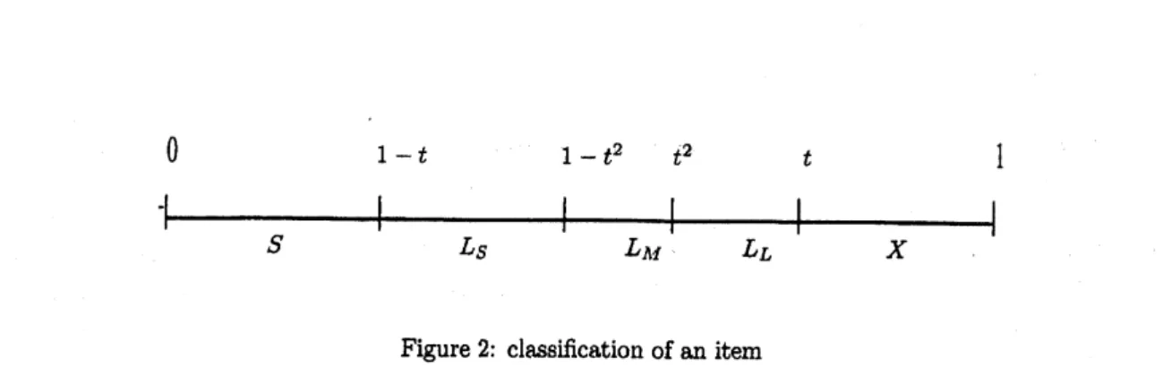
Each item satisfies:
$0<|s|\leq 1-t$
,
$1-t<|\ell|\leq t$
,
and
$t<|x|\leq 1.$
Now
we
explain
how to devide items. If
a
player
can
make
a
bin larger
than tlle
size
$t$,
it is clear
that
$CR$
of
this
case
can
satisfy
$CR$
$<\alpha$
.
If
a
item
of
$X$
is
given at the
first
time,
a
player
carx
make
the
good
bin with
only
$x$
.
Therefore,
we
think
only the
case
where
no
items
of
$X$
are
given.
That
is,
a
class
$X$
is designed
so
that
we can
ignore
the
class
$X$
as
inputs. Next,
we
discuss
a
class
$S$
.
If
a
$\ell_{S}$must
be
discarded,
Each size
of
all
bins
a
player has is larger
than
$t$
.
Then,
the
player
satisfies
$CR<\alpha$
.
Therefore,
we
think also only the
case
where
no
items of
$X$
are
given.
That
is,
$O$
is designed
so
that
we
can
think only
a
class
$L$
as
inputs alld
if
the
player
can
make
the
bin larger
than
size
$t$
,
the player
just
discards
given items
after that.
By
the way,
we
describe
a
primary principle
to
determine which
$\mathrm{i}\mathrm{t}\mathrm{e}$ms are
discarded. The
principle is to
substitute
a
smaller
item
for
a
larger item. That
is,
if
a
player
discards
a
item,
the player keeps
a
$\mathrm{s}$maller
item
than it
to substitute for
it.
But if
a
item is
by
far smaller than the
other,
it
cannot
be substituted for a
larger
one.
To substitute
$v$
for
$u$
,
$u$
and
$v$
must
satisfy
the
following conditions.
.
$|v|\leq|u|$
(Otherwise,
the adversary
gives
an
item
whose size
is l-[ul
as an
input, alld
a
player
$\mathrm{r}:\mathrm{a}\mathrm{n}\mathrm{n}\mathrm{o}\mathrm{t}$hold
the
item.)
.
$\Pi v|u|<$
a
(Otherwise,
the adversary
stops inputs. If
the
size
of
offline
and online
are
$|u|$
and
$\rfloor v|$
,
respec-tively,
a
player cannot satisfy
$CR$
$<\alpha$
.)
That
is,
if
a
player
discards
$u$
,
the
player
must
keep
$v$
which satisfies the above
conditions.
To satisfy the the above
substitution
conditions,
$L$
is
devided
into
more
three different
classes
$Ls\cdot L_{\mathrm{A}}$
,,
and
$L_{L}$
, shown in
Fig.2.
An item in each class
is
denoted
by
$\ell_{S}$,
$\ell_{M}$
,
and
$l_{L}$
, respectively. Each item satisfies:
$1-t<|\ell s|\leq 1-t^{2},1-t^{2}<|\ell_{\mathrm{A}I}|\leq t^{2}$
, and
$t^{2}<|\mathit{1}_{L}|\leq t.$
Because
of
$\lrcorner_{\mathrm{A}}\ell p,$,vn\iotaih,L\iota
$<$
$\mathrm{f}\mathrm{i}$$=\alpha$
,
$\ell_{L\min}$
cau
substitute
for
all
$\ell_{L}$’s
so
far
given.
That
is,
$L_{L}$
is
a
$\max$
range
which
can
substitute
for
an
item of size
$t$
.
A
$\ell_{\mathrm{A}\mathit{1}}$aazd
a
$\ell_{L}$
cannot be hold in the
same
bin at the
same
time,
because the total of lower bounds of
$L_{\Lambda \mathit{1}}$
and
$L_{L}$
is
over
1.
Moreover,
a
$\ell s$
and
a
$\ell_{M}$
can
lee
hold in the
same
bin at the
same
time unconditionaly, because the total
of
upper bounds of
$Ls$
and
$L_{M}$
is
under 1.
Furthermore,
we
focus
on
whether
a
group of
classes is
over
$t$
,
or
not,
and regard
$2t-1$
and
$2-2t$
as bounds
72
0
$1-t$
$1-t^{2}$
$t^{2}$$t$
1
Figure
2: classification of
an
item
3.2.2
Online
Algorithm
for
$\alpha\approx$1.3660
Next,
we
discuss
an
online
algorithm
$O$
where an
input
$\alpha$is
$\frac{1+\sqrt{3}}{2}(=\alpha\approx 1.3660)$
.
$t$
is
a
$111\mathrm{a}\overline{\lambda}$
point
$\mathrm{w}1_{1}\mathrm{i}\mathrm{c}1_{1}$satisfies
$\frac{t}{2-2t}<\frac{1}{t}=\alpha$
.
That
is,
$t$
is
one
of
the roots
of
each
equation
$2-2t=t^{2}$
azxd
$2t-1=1-t^{\underline{)}}$
.,
and
$t$is
$\sqrt{3}-1.$
Items of
each
class satisfies:
$\frac{3-\int\overline{3}}{2}(\approx 0.2679)<|\ell s|\leq\frac{\sqrt{3}}{2}(\approx 0.4641)$
,
$\frac{t3}{2}<|\ell_{t}$
,
$| \leq’\frac{\sim-\sqrt{3}}{2}(\approx 0.53_{\mathrm{J}}^{r}|9)$
,
and
$\frac{2-\sqrt{3}}{2}<|l_{L}|\leq\sqrt{3}-$
$1(\approx$
0.7312
$)$.
Let
$N(c)$
be the
$\max$
number that
a
player
can
hold items
of
a class
$c$
in
the
sam
le
bin
at
the
same
time.
For
exmaple,
$N(L_{L})$
,
$N(L_{M})$
, and
$N(Ls)$
are
1, 2, 3, respectively. The number that
items
of
a
class
$c$
.
call
component
the
size of offline
is
at most
$N(\mathrm{c})$
.
Therefore,
a
player
may
hold at most
$N(c)$
items of
a
class
$c$
.
at
the
same
time.
In
$L_{L}$
,
because
$N(L_{L})$
is
1 and
$L_{L}$
is a
$\max$
range
which
can
substitute for
an
item of size
$t$
,
a
player
ulay
hold at least the smallest item
of
$\ell_{L}\mathrm{s}$so
far
ever
given. In
$L_{M}$
,
though
$N(L_{\mathit{1}\}l})$
is 2,
when
a
player
has two
$\ell_{M}\mathrm{s}$
in
a
state,
the two items cannot be hold in the
sa ne
bin at the
same
time. Therefore, the number that
items of
$L_{M}$
call
component
the size of offline is
at
most
1,
and the
player
may hold at
most
one
item of
$L_{\mathrm{A}\mathit{1}}$at the
same
time. Because of
$\lrcorner\ell\ell_{M\mathrm{n}1i,\iota}^{1\mathrm{r}\mathrm{u}h\angle}<\neg 1-tt^{2}<\alpha$, a
player
may
also hold at least the smallest item of
$\ell_{\mathrm{A}\mathrm{f}}\mathrm{s}$so
far
ever
given.
In
$L_{s}$
,
For
a
similar reason,
a
player
may
also
hold at least the smallest and the second
smallest items of
$\mathit{1}s\mathrm{s}$so
far
ever
given.
After
all,
a
player
will substitute
a
smaller item for a larger item
in
the
salrie
class. That
is,
if
a
player
must
discard
an
item
of
a
class,
the
player will
discard
a
larger
item
of
the class and
keep
a
smaller item of
the class.
3.2.3 Online
algorithm for
$\alpha\approx$1.3333
$t= \frac{1}{\alpha}$
means
that
$CR$
is
improved
if
$t$
is larger.
Therefore,
we
aims
at designing
0
which has
larger
$t$.
We
designed
$O$
which has
$t= \frac{3}{4}$
.
That
is,
We
improved
$O$
so
that
$O$
satisfies
$CR< \frac{4}{3}$
$(\approx$1.3333
$)$.
Tbe
classification
of items
is
shown in Fig. 3.
$L_{J_{1}\mathit{1}}$,
is
devided into
more
two
different
classes
$L_{\mathrm{A}IS}$and
$L_{\Lambda \mathit{1}L}$-0.25
0.4375
0.5
0.5625
0.75
Figure
3: Classification
of
the
items according to
their
sizes.
substitute
for
$\ell_{ML}$
.)
But it
is
not enough. Therefore,
we can
think
to substitute two
or
$\mathrm{r}$
ore
items for
one
item. For
example,
To substitute
$v_{1}$and
$v_{2}$
for
$u$
,
$u$
and
$v_{1}$alld
$v_{2}$
must
satisfy the
following conditions.
.
$|v$
)
$|+|v_{2}|\leq|u|$
(Otherwise,
the adversary
gives
an item whose
size is
$1-|u|$
as
an
input,
and
a player
cannot
hold the
item.)
.
$\frac{|u|}{|v_{1}|+|v_{2}|}<$
’
(Otherwise,
the adversary stops
inputs.
If the size of offline and online
are
$|u|$
and
$|\mathrm{t}_{1}’|+|v_{2}|$
,
respectively,
a
player
cannot
satisfy
$CR<\alpha$
.)
We design
$O$
so
that two items of
$Ls$
substitute for
a
item of
$L_{L}$
.
The
subs titution
happens
when
two items of
$Ls$
and
one
item
of
$L_{L}$
are
held and
one
or more
items must be
discarded.
If
the subtitution
happens.
0
can
satisfy the above second conditions
surely. Therefore,
$O$
must
satifsy
the above first conditions to
substitute.
That
is,
when
there
is
a
possibility
to
substitue two
$\ell s\S$
for
one
$\ell_{L}$,
if
$|\ell s|+|?s|\leq|\ell_{L}|$
holds,
0
discard the
largest item of
$L_{L}$
and
keep
items
of
$L_{S}$
,
otherwise,
discards
the largest items of
$L_{S}$
and keep items of
$L_{S}$
.
3.3
Algorithm
$A$
3.3.1
Outline of Algorithm
$A$
$A$
is
a
part
of
$A_{ey\mathrm{A}em}$
, and exist to make state transitions. When
a
item is
given in
a
state
as
an
input,
it
happens
a
transition from the state.
$A$
outputs
the transition state.
As
inputs,
a
state and
one
of the
classified
classes which
are
given
to
$A_{system}$
are
given
t)
$A$
.
Then,
$A$
makes the transition and
new
conditions which
states have, and output the transition
state.
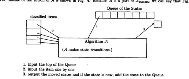
The outline of the action
of
$A$
is
shown
in
Fig.
4.
Because
$A$
is
a
part
of
$A_{syster}$
,
we can
say that
Fig.
$\ovalbox{\tt\small REJECT}_{\mathfrak{B}\mathrm{t}\mathrm{e}\mathrm{a}\mathrm{n}88}^{\mathrm{l}}\mathrm{a}s\mathrm{s}1\mathrm{f}\mathrm{i}\mathrm{e}\mathrm{d}\mathrm{t}\mathrm{e}\mathrm{m}\mathrm{s}\ovalbox{\tt\small REJECT} 1\mathrm{e}\mathrm{b}\varphi$
1.
input
the
top
of the
Queue
2.
input
the item
one
by
one
3.
output
the moved states and if the state
is new,
add the state to the
Queue
Figure
4:
Outline
of
an
algorithm
$A$
.
4 shows
a
part
of
actions
of
$A_{*ystem}$
.
There is also
a
queue of the states
in
$A_{\theta yste’ n}$
.
Of course, the queue
includes
only
an
empty
state
at
the first time. As
inputs,
the
top
of the queue
and
one
of the
classified
classes
which
are
given to
$A_{sy\epsilon \mathrm{t}em}$are
given
to
A.
(Each
classified class is
given
one
by
one
to
one
state.)
Then,
$A$
makes
a
transition
state,
and
outputs
it.
If
the
state
is
new, then it is added
to
the
bottom
of
the
$\mathrm{q}^{\mathfrak{l}}$ueue.
The
actions
are
continued till the queue is
empty.
All states which
are
made by
$A$
have
conditions,
and given
to
74
3.3.2 Structure
Next,
we
discuss the structure of the algorithm
$A$
.
We know that
$A$
is
given
one
state
and
one
classified
item
as
inputs
and makes
a
transition state which has
conditions, using them,
from the above
arguu]ellt.
Now,
we
describe how
to
make
a
transition
state.
Each class has
a
upper and lower
bounds,
and let
a
item of
the
class be
$u$
.
$A$
makes
new
conditions and a
transition state, using
Wi,
$W_{2}$
,
$u$
,
conditions
and
their
bounds. The flow chart of
$A$
’s
action
is
shown
in
Fig.
5.
Firstly,
$A$
checkes
whether there exists
a
group which
can
make the bin
more
than
$t$with
$\prime u$$\cup \mathrm{t}\dagger_{1}.\cup \mathrm{f}!V$2
unconditionaly
or
not.
If
the
classification is
like
Fig.
3,
two items
of class
$\ell_{\mathrm{A}IS}$or
each
one
item
of
class
$p_{g}$
.
and
$\ell_{h\mathit{1}L}$constitutes such a group.
If there
exist,
$A$
outputs EndState. Otherwise,
A goes to the
next
cheek.
The
next
check
is
whether
there exists
a group
which
can
satisfy
both the total
of their
lowerbound
is at
least
$t$
and the
total of
their
upperbound
is
at most
$t$
,
or
not. Now, if
there exists
a
group which can
make
$\epsilon\iota$bin
smaller
than
$t$
, we
think the
group
cannot
exceed
$t$.
For
example,
if
there exists two
$\ell s\mathrm{s}$
in Fig.
3,
we
think
$|\ell s|+|\ell s|\leq t.$
Therefore, if
there
exists,
$A$
adds
the
new
conditions with the
output
state and go to
the
next
check. Otherwise,
$A$
goes
to the next check without adding the
new
conditions. For
example,
two
$\ell_{S}’$’s
can
do
in
Fig. 3. The
new
condition,
$\ell s+\ell s\leq t,$
is added to the
output
state. The next check
is
whether
there exists
a
group which
can
satisfy both
the total
of
their lowerbound
is
at
least
1 and the total
of
their
upperbound is at
least
1,
or
not.
If there exists,
$A$
adds the
new conditions
with the output state and
go to
the next check.
Otherwise,
$A$
goes
to
the next check
without
adding
the
new
conditions. For
example,
three
$\ell s’ \mathrm{s}$
can
do in
Fig.
3. The
new
condition,
$\ell s+\ell s+\ell s>1,$
is
added to the
output
state. The next check
is
whether
$A$
can
put
$u$
into bins,
discarding
no
items
, unconditionaly,
or
not.
For
example,
tlxe
case
i
$\mathrm{n}$
which
the item
of
$\ell s$is given in
the
state3
of
Section 3
does. If
the
player
carl
do,
the state which
is
put
the class
from
the
input
state
is output.
Otherwise,
$A$
must
discard
one or
more
items. Therefore,
$A$
determines the
removed
items and
output the transition
state. Determining
the
removed
items is
very
importan for this
system.
This
action changes
with
online algorithm
$O$
given
as
an
input.
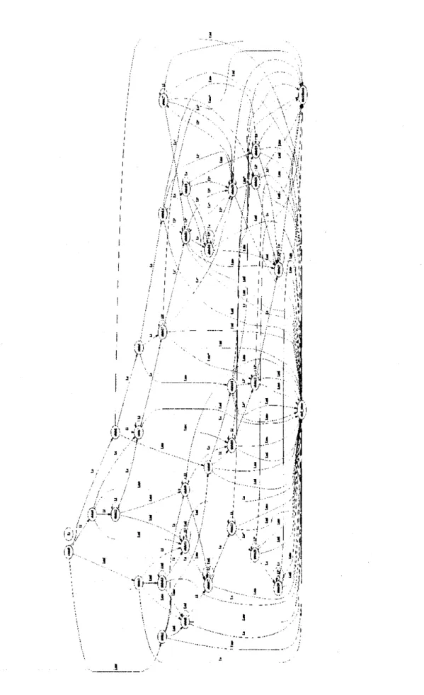
3.4 Results
We
have applied
algorithm
$A_{system}\mathrm{f}\mathrm{o}\mathrm{r}$the
two
online
algorithms of
EOK and obtained
the
following
$\mathrm{L}^{\cdot}\mathrm{O}\mathrm{I}\mathrm{I}\mathrm{I}-$
petitive
ratios.
Figure 6 illustrates the state transtion of
the online
algorithm of
$ce\approx$
1.3333 obtained
by
$A_{syst\mathrm{e}m}$
.
The state
transition
and the competitive ratios of each state is confirmed
automatically.
Theorem 1 The online
algorithms
in Section 3.2. 2
and
3.2.3 have the
competitive ratios
$\alpha\approx$
1.3660
and
1.3333, respectively.
4
Concluding
Remarks
In
this
paper,
we
studied
an
automated
competitive analysis
for the exchangeable online knapsack
problem.
We
showed
proofs
of
$i$
he upper
bounds 1.3660
and
1.333
for 2-bin
EOK. Although
there
is
a gap
between the
lower and
the
upper
bounds,
our
results
give
a
basis
for the
tight
bound. The bounds for
$k$
-bin EOK should
State
$\Leftarrow$iten
can
ma
$\mathrm{t}\mathrm{e}$ore
$1\mathrm{t}$an
ere
.
$\mathrm{t}$a
$\mathrm{r}\mathrm{o}\mathrm{u}$ $\mathrm{Y}$
output
$\mathrm{E}$state
$t$
uncon
ltlona
$\mathrm{y}$.
$\mathrm{N}$
$\mathrm{e}\mathrm{e}$
.
$\mathrm{t}\mathrm{s}$a
$\mathrm{r}\mathrm{o}$ $\mathrm{h}\mathrm{i}\mathrm{c}$ $\mathrm{Y}$add
new con
.tions
to
the utput
tate
$\mathrm{s}\mathrm{t}$
0
$\mathrm{t}$ $\mathrm{o}\mathrm{t}$of
$\mathrm{t}\mathrm{e}1$ $\mathrm{o}^{\mathrm{O}\mathrm{W}}\mathrm{r}\mathrm{o}$$\mathrm{d}>t\mathrm{n}$
the tota
the
group
$\leq t$
$\mathrm{r}$
upper
oun
$<t$
.
$\mathrm{N}$$\mathrm{e}\mathrm{e}$
.
ts
a
rou
whic
$\mathrm{Y}$add
new
conditions
the
utput
$\mathrm{t}$.
$\mathrm{o}\mathrm{a}\mathrm{n}\mathrm{s}\mathrm{r}\mathrm{t}\mathrm{i}\mathrm{s}\mathrm{o}\mathrm{l}\cdot \mathrm{u}\mathrm{p}\mathrm{p}\mathrm{e}\mathrm{r}\mathrm{o}\mathrm{u}\mathrm{d}\mathrm{o}\mathrm{u}\mathrm{n}\mathrm{l}\mathrm{a}(\mathrm{t}$
$0$
le.
oftota
$\mathrm{e}1$the
group
$>1$
$\mathrm{N}$er
ca
put
$u$
in
isca
$\mathrm{g}$no
iten,
uncon
ltlona
.
$\underline{\mathrm{N}}$$\mathrm{Y}$
hold
ite
\sim \sim \sim \sim ----\sim \sim -\sim \sim --\sim -\sim \sim
$\sim\sim\sim\sim-’$,
”
determine
the removed ite
and
,”
$l,\mathrm{o}\mathrm{u},\mathrm{t}\prime \mathrm{p}\mathrm{u}\mathrm{t}\mathrm{t}\mathrm{h}\mathrm{e}\mathrm{t}\mathrm{r}’-\prime\prime\sim\sim\sim\sim--\sim\sim\sim\sim-\sim-,-\mathrm{i}\mathrm{t}\mathrm{i}\mathrm{o},\mathrm{t}\mathrm{a}\mathrm{t}\mathrm{e}--\sim--\sim--\cdot--\sim-\sim\sim-\sim-\wedge$
output
$\}$
$’|$
$\mathrm{t}_{l_{\backslash }}^{3}|\backslash \acute{\downarrow}$
.
- -$\underline{1}-$,
$\mathrm{t}$.
j-.,
$||$!
$\underline{\backslash }$ $\mathrm{t}^{\dot{\mathrm{A}}t}’|$!
$\mathrm{i}$’
$|$ $||$$j_{\mathfrak{l}}|,’\acute{j}_{1}\prime\prime.,‘ j\underline{\backslash }\prime j^{\frac{}{\mathrm{i}_{1}}}||.\backslash .\cdot 5$ $-\sim|$
;.}’
$\underline{\neg.}-\vee-\underline{\backslash 1}-\prime_{*k}\grave{1}_{\backslash }i.\mathrm{i}_{\mathrm{J}}^{1}|$
$|$
$|$
$!\mathrm{i}^{\backslash 1}\iota\cdot’\prime 1_{1}^{1}|\backslash$
.
$\mathrm{I}.\underline{\backslash }$,
$‘ f’\backslash \backslash$ $\backslash .\underline{\neg.}$,
$|$ $||$ $\dot{I}_{\overline{]}\acute{)}\mathrm{a}_{1}}^{\mathrm{I}}\mathrm{t},’\backslash$,{‘t
$.4,|\backslash \prime\prime\backslash$ $||$ $\backslash \grave{\prime}.$’
-1
$s$.
$\underline{\mathrm{B}}1$ $|$,
$j\backslash$ $|||$ $\underline{\backslash }$’
$|$ $|’|$$;\{$
$\underline{\mathrm{r}\mathrm{I}}|$ $||$$t3$
$’|,\mathrm{i}\prime 1--$ – $\underline{1}-_{\underline{1}-}’|\rceil|$’
$\prime 1_{\mathrm{s}}|3$ $|^{\prime t}2$.
r
$s-_{\underline{\mathrm{I}}}^{\underline{\underline{1}}}---. \frac{\backslash }{s}]_{\mathrm{I}}^{\}^{\mathrm{a}_{\mathfrak{l}}}}-\acute{\grave{\mathrm{i}}}_{f}3^{\cdot}\prime 1|i_{\grave{\mathrm{t}}}\acute{|}$
}
$\}$
$t|$
$l_{J}^{\backslash }\ddagger 1^{1}\backslash \cdot+_{\backslash }’-\backslash 1$
$s \backslash ;\neg-i_{\backslash }^{\mathrm{f}_{j}}\oint_{\sim},\backslash ^{\mathrm{J}}$
‘
$1$ $s$ ”1
$.\cdot\backslash$ $\backslash \backslash 1\backslash \backslash$’
$r_{\mathrm{r}^{l},*\mathrm{I}!1},\mathrm{r}_{\mathrm{I}},\{\mathit{1}l$
.
$,|$
$||.\backslash \backslash \prime \mathfrak{x}_{\downarrow,\mathrm{Y}\backslash ^{1}}.\grave{\mathfrak{s}}^{1}\mathrm{I}|_{1}^{||}\backslash ’ d’‘\downarrow..,\cdot.\overline{\mathrm{I}}\backslash i_{9}^{\backslash _{5}}|\acute{\iota}^{\dot{1}}\mathrm{b}\mu_{\mathrm{t}^{-}}\backslash t\prime_{1}^{\mathfrak{i}}|1_{1}’\frac{:\dot \mathrm{f},}{}\backslash \backslash \dot{\mathrm{a}}\mathrm{I}r\iota|1|_{1}^{\mathfrak{i}_{\backslash u}^{\mathrm{f}^{1}}}_{\mathrm{I}}’.‘..\mathrm{i}|\backslash \prime^{\backslash }|j\mathrm{e}i_{1}’|||||!\downarrow\acute{1}1\dot{\mathrm{i}}_{\mathrm{t}}1_{\mathrm{t}}^{/}\iota||_{1_{1}}|\prime \mathrm{r}_{\mathrm{I}}^{\mathrm{I}’}||\mathrm{i}$
;
$||^{1_{\mathrm{i}}^{1}}$}
$|||$ ’$.\backslash s$,
$\cdot.\mathrm{t},\cdot.\int_{\grave{\backslash }i}^{1}1||\downarrow,,\mathrm{J}|^{\underline{\eta}|}\backslash |*|$’
$|_{\mathrm{I},\lrcorner}.\cdot.1.,\cdot.’\cdot‘ \mathrm{I}_{\{}|_{\mathrm{I}^{t}}-\sim..\iota_{\mathrm{t}^{\backslash }.\prime\cdot\prime_{1}}^{\mathfrak{l}1^{1}}s_{\grave{\mathrm{i}}\mathrm{I}^{1}.\{^{\mathrm{t}}}^{t^{\backslash }\frac{\mathrm{I}}{1}}\prime \mathrm{r}_{1}^{\underline{\mathrm{I}}}|\downarrow \mathrm{b}^{1^{||}}|\dot{3}_{\sqrt\dot{\mathrm{i}}}\iota_{\theta^{\downarrow}}|/:_{l}^{1}!_{1}^{-}\wedge-|\}\}_{\backslash }||.|‘..\cdot\iota_{1}1-^{\mathrm{I}}\wedge l\mathrm{i}\backslash |’|||\backslash \mathrm{t},|\iota^{1}1^{1}\mathfrak{l}|\ovalbox{\tt\small REJECT}^{1}1|r_{l}^{!}|||\mathfrak{l}^{\iota}\mathrm{t}\mathit{1}|\backslash 1\mathrm{h}||\mathrm{J}^{1}$
.
-,–1
$\cdot$$\mathrm{E}$
$\sim.- \mathrm{t}^{-}..\cdot.-|_{d}1--;,\dot{0}^{\mathrm{v}_{1}}r\}_{1}\iota 1\oint^{1^{1}}1\underline{|}.\cdot$
$\mathrm{j}$ $\backslash |\grave{1}^{\mathrm{t}}\backslash ’$
’. $.–|$
–
$\underline{1}$$[^{-}-$
}
$|||\{l$$11$
$\sim,|\mathrm{i}_{C}^{\backslash }’\neg$,
$|.|$ $\mathrm{s}_{--}$:.
$\underline{\prime}$1|
– $:\dagger \mathrm{t}^{1}$$1:’$
;
1
$\backslash \mathrm{k}\aleph..|\underline{\lrcorner\overline{1}}j\backslash -\backslash -\prime \mathfrak{l}|||\mathrm{l}\mathrm{i}11$ $|\mathrm{t}|||^{1}\|’||^{1}$’
.
$\underline{\neg}j(.1.\cdot j\overline{\mathrm{q}}j$$!$
’
$.(1.j\overline{\mathrm{q}}\mathrm{i}$ \dot $\mathrm{i}\overline{\grave{1}}j\backslash --\cdot$;
$\mathrm{a}.j$.
$\neg\prime r\underline{-}’\underline{\sim\backslash }\sim\backslash \{\backslash ^{\downarrow\backslash },\underline{\iota}\overline{\mathrm{f}}^{\iota^{J}}$
.1
$.-\cdot/$ $\theta\backslash ^{l}\mathrm{I}_{\mathrm{c}_{\vee}}\dot{\grave{1}}$
$>^{y}3$
$\mathfrak{g}^{\dagger}||$
$\sim\backslash \cdot\overline{t^{\mathrm{I}\sim}|}|\iota_{!}.,|’|.\mathfrak{g}|\vdash-\neg.1^{\backslash }\mathfrak{l}_{\dot{|}}\mathrm{i}\iota_{!}^{1}\mathrm{r}$ $’|\underline{:}$
,
$\underline{\backslash }$.
$—-\vee 411---\cdot$
1
$’|$ $.l|||!$1
$1|${
$/\backslash .1_{\backslash }\epsilon_{i}^{\overline{-}}$,
$\cdot$ $d$ $\psi_{\mathrm{s}^{\mathrm{Y}}}^{\tau f1}.\mathrm{r}_{l}s^{1}$.
:
$|$:
$i$;
$||$.\dagger’’
$\backslash *\backslash 1^{t}\vdash_{\backslash }$$\sqrt$