Mining Association Rules using Lattice Theory (6th Workshop on Stochastic Numerics)

122

Mining

Association

Rules

using

Lattice

Theory

Florent

Domenach

Masato Koda

Institute ofPolicy and Planning Sciences,

Tsukuba University,

1-1-1 TennO-Dai,

Tsukuba, Ibaraki 305-8573, Japan,

$\mathrm{e}$-mail : {domenach,koda}@shako.sk.tsukuba.ac.jp

Tsukuba University,

1-1-1 TennO-Dai,

Tsukuba, Ibaraki 305-8573, Japm.

$\mathrm{e}$-mail:{domenach,koda}@shako.sk.tsukuba.$\mathrm{a}\epsilon.\mathrm{j}\mathrm{p}$

Abstract

The problem ofdiscovering nontrivial association rules from large

databases has recently become critical, especially 01 data mining area

where there exists a substantial need to develop efficient mining

al-gorithms for complex data. In this paper, we consider the situation

where items are constrained, i.e., some taxonomies (or hierarchies) on

theitems areknown. Wefirst show howtaxonomies canbegeneralized using lattices, which are ordered structures, to represent constraints

on items. Then, we propose a new approach to find association rules,

based on the notion ofbiclosures introduced by the first author.

Keywords: Association Rule,

Galois

Connection, Implication, Lattice.

1

Introduction

Data Mining is essentially done using statistical and computational

tech-nics (e.g. principal component analysis, factor analysis, $\rangle$

.

), to reveal

hid-den factors that underlie sets of variables, measurements

or

signals. In

a

more

algebraic approach,

Galois

connections first provide the mathematical

formalization of

the classical $\mathrm{e}\mathrm{x}\mathrm{t}\mathrm{e}\mathrm{n}\mathrm{t}/\mathrm{i}\mathrm{n}\mathrm{t}\mathrm{e}\mathrm{n}\mathrm{t}$ scheme of objects

described

by

properties (see,

e.g.,

[4, 12, 17]).

Given

a

relation between

a

set of objects and

a

set of properties, dually isomorphic orders

on

classes of objects and

sets of shared properties

are

provided by

a

natural Galois connection. This

basic fact

was

then frequently rediscovered in the literature. Combined with

other considerations, it

was

successfully developed in Formal Concept

123

Theory, Conceptual Classification, Relational or Object Databases (see, e.g.,

[7, 18, 23, 29]$)$

.

They have been recognized

as a

fundamental mathematical concept in

the middle of the century ([5, 15, 26]), and constitute

a

useful tool in

se-veral domains

related

with data analysis like modelization and aggregation

of similarities and preferences ([19, 21, 22]) or mathematical morphology ([20]). They

are

strongly associated to many fundamental notions: among

others, closure operators, full implicational systems [2], and,

more

recently,

overhanging relations [10].

In the applications domainsmentioned above, there is

a

need for efficient

ways of handling and transforming Galois connections. In that purpose, af-ter recalling

some

basic definitions in Section 2,

we

will present here, in

a

latticial oriented approach, different DataMining tools, such

as

implications

and their generalization, the

association

rules (Section 3). Finally, in

Sec-tion 4,

we

will introduce what

we

mean

by conceptual classification with

constraints.

2

Definitions

First let’s recall

some

basic definitions, together with some well known

pr0-perties about closure mappings, lattices and Galois connections.

2.1

Closure Mappings

and

Lattices

Let $S$ be

a

finite set.

A

closure space is

a

pair $(S, \varphi)$

,

where _/’ is

a

closure

operator

on P

$( \mathrm{S})$

,

that is

a

mapping onto $P(\mathrm{S})$ satisfying the following three

properties:

(C1) $\varphi$ is isotone: for all $A$,$B\subseteq S$,$A\subseteq B$ implies $\varphi(A)\subseteq\varphi(B)$;

(C2) ip is extensive: for all $A\subseteq S$, $A\subseteq\varphi(A)$;

(C3) $\varphi$ is idempotent: for all $A\subseteq S$

,

$\varphi(\varphi(A))=\varphi(A)$

.

The image $\mathcal{F}_{\varphi}=\varphi(7(S))$ of$P(S)$ by ? is exactly the set of all the fixed

points of $\varphi$

,

which

are

called the elements of $P(\mathrm{S})$ closed by /2.

A

lattice is

a

tuple $(L, \vee, \wedge)$

,

where $L$ is

a

set, $x\vee y$ is the lowest

upper

bound of$x$ and$y$ and$x\wedge y$ is the greatest lower bound of$x$ and$y$

.

These two

operators

are

also called respectively join and meet of $x$ and $y$ (for further

information

on

lattices,

see

$[5, 11])$

.

With the inclusion order, $(\mathcal{F}_{\varphi}, \vee, \cap)$ is

also

a

lattice with $\vee X=\varphi(\cup X)$ for $X\subseteq \mathcal{F}_{\varphi}$

.

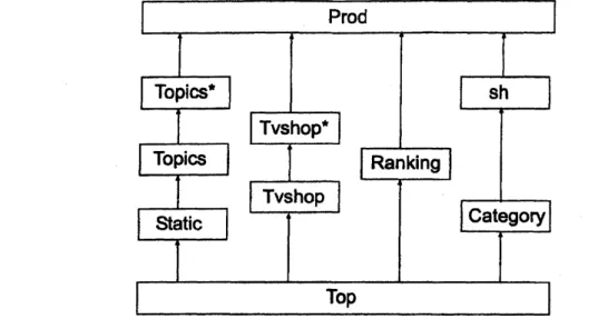
By the extensivity property,

Example 2.1 A web site selling products

can

be modelled in the following lattice (Figure 1), the minimum element being the home page, and the

ma-ximum the page where the products

are

sold.

Figure 1: Lattice of a web site.

Example 2.1 Let $\prime H$ be

an

hierarchy

on

_$S$, that is

a

set of subsets of _$S$

(clusters) satisfying the conditions: (HI) $S\in lt,$ (H2) for $H$

,

$H’\in H,$$H\cap$

$H’\in\{\emptyset, H, H’\}$, and (H3) for all $s\in S$, $\{s\}\in$ ?t. The set $H$ $\cup\{\emptyset\}$ is

a

closure system

on

$S$

.

Hierarchies constitutes

a

basic model ofclassification

trees.

Conversely,

a

closure $\varphi_{F}$

on

$P(S)$

,

given by $\varphi_{F}(F)=\cap\{F’\in$ $t$ : $F\subseteq$

$F’\}$

,

corresponds, in this way, to any family

7

of subsets of$S$ satisfying (i)

$S\in \mathcal{F}$

,

and (ii) $2”\subseteq$ I implies $\cap \mathcal{F}’\in$ $\mathrm{r}$

.

With these properties, $\mathrm{F}$

is saidto be

a

Moore family (or

a

closure system)

on

$S$

,

and

we

denote by $\mathcal{M}$ the set

ofall Moore families

on

$S$

.

It is well-known that Moore families and closure

operators

are

in one-t0-0ne correspondence and constitute in fact equivalent

notions. The set $\mathcal{M}$, ordered by inclusion, is itself

a

lattice, whose main

properties

are

described in the recent work of [6].

An

element $j$ of the lattice $(L, , \wedge)$ is join irreducible if $X\subseteq L$ and

$j=\vee X$ imply $j\in X;$ the

set

of

all

join

irreducibles

of

$L$ is

denoted

as

$J_{L}$

or

$J$ if

no

confusion is possible. The join

irreducible

elements of$L$

are

those

which cannot be obtained by others and using thejoin operator. Dually,

an

element $m$ of $L$ is meet irreducible if $X\subseteq L$ and $m=\Lambda X$ imply $m\in X.$

The set of all the meet irreducibles of $\mathcal{F}$ is denoted

as

_{$M_{L}$}

or

$M$

.

For

an

125

are

respectively called the principal ideal and the principal

_filter

of $L$ with

basis $x$

.

2.2

Galois

Mappings

Let $L$ and $L’$ be two complete lattices, and

a

mapping _$f$ : _{$Larrow L’$}

.

A

mapping satisfying the following condition is said to be

a

Galois

mapping

([26]) :

(GM) the mapping $f$ is antitone and there eists

an

antitone mapping$g$

from

$L’$ to $L$ such that the composition mappings

$\varphi$ $=gf$ and $\psi$ $=fg$ are

extensive.

The pair $(f,g)$ is

a

Galois _connection between $L$ and $L’$; the maps _$fyg$

in

a

Galois connection determine each other uniquely. Both composition

mappings / and $\psi$

are

closures, respectively

on

$L$ and $L’$

.

The ordered sets

$\mathrm{X}$

$=\varphi(L)$ and $\mathrm{I}=\psi(L’)$

are

dually isomorphic by the restrictions of$f$ and

$g$

.

The following type of Galois connection is fundamental in data mining.

Consider two sets $S$,$A$ and a relation $R\subseteq S\mathrm{x}A$

.

For example, $S$ can be a

set of objects, $A$ a set ofattributes and $R$ is the relation $sRa$defined by ”the object $s$ has the attribute $a$” For $s\in S$

,

$a\in A,$ the equivalent notation $sRa$

or

$(s, a)\in$ ff will be used according tothecontext. Define$f_{R}$ : $\mathcal{P}(S)arrow P$(A)

and $g_{R}$ : $P(A)arrow$ $P(\mathrm{S})$ by $f_{R}(C)=$

{

$a\in A:(s,a)\in R$ for all $s\in C$

}

and $g_{R}(D)=$

{

$s\in S$ : $(s,$$a)\in$ R for all $a\in D$

},

for all $C\subseteq S$

,

$D\subseteq A.$

The mapping $f$ associates to

a

set

of objects $C$ all the

attributes

shared

by all the objects in $C$

,

the intension of $C$

,

and $g$ associates to

a

set of

attributes $D$ all objects having all the attributes in $D$

,

the extension of

$D$

.

It is straightforward that the pair $(f_{R}, g_{R})$ satisfies Condition (GM) and

constitutes

a

Galois connection between $P(S)$ and$P(A)$, bothendowed with

the inclusion order. The lattice of closed subsets of$S$ is the Galois lattice of $R$, sometimes also called (formal) concept lattice.

Example 2.3 Set $P=P$(S), where $S$ is the finite set of objects under

study, and consider

a

(complete) lattice $Q$ of descriptions, together with

a

description$d(s)\in Q$ of each element $s\in S.$ The order of$Q$ corresponds with

a

generalization order, where $q\leq q’$

means

that description$q$

is

more

general

than description $q’$ (an example of such

a

lattice is the

one

ofExample 2.1).

Then, it is said that $s\in 5$ satisfies description $q$ if $q\leq d(s)$

.

For any class

$C\}$ and $g(q)=\{s\in S : q\leq d(s)\}$ constitutes

a

Galois connection between

$P(S)$ and $Q$

.

Remark 2.1 Example

2.3

can

appear to be

a

generalization of the previous

type of Galois connection; in fact,

as

shown in [17], the Formal Concept

Lattice scheme is the

more

general

case

(see [9] for

a

presentation of

a

common

frame).

The well-known Galois connection associated with the

table of

finite

lattice $T$ belongs to the previous type. The table of $T$ is the relation $R\tau$ $\subseteq$

$J\mathrm{x}M$ defined by $(j, m)\in R_{T}$ if$j\leq m,$ for any $j\in J$

,

$m\in M\mathrm{r}$ Every finite

lattice is isomorphic to the Galois lattice associated with its table ([4]). The generalization of this fact to any complete lattice

was

given by [30].

2.3

Galois Connections in Data

Mining

One basic purpose

of any Data Miningis to obtain classes of objects sharing

similar characters,

a

description by attributesbeing associated to each class.

As

described above, Galois connections, by providing

a

correspondence

be-tween extents and intents, satisfy this purpose.

Another important aim in Data Mining is to organize data to make it

more

readable

or

to

recover

some

unknown structure. For instance,

hier-archical clustering methods provide

a

classification tree, sometimes (e.g. in phylogenetic reconstruction

or

cognitive psychology)

an

estimationof

an

un-knowntree. TheGalois lattice does not correspond to such

an

objectivesince

it

preserves the

whole

information

of the data. So,

as ffequently

observed

in the literature, it has

a

great sensitivity to noise and deviation from the

model. Also, the number of concepts potentially grows exponentially with

the data size, leading to problems of computational complexity.

Between many different approach,

one can

pick methods to prune the

concept lattice, for instance by limiting its construction to a convenient

filter [24]. Another approach,

more

practically oriented, is to consider

wea-kened conditions for the closure systems associated,

or

for the (equivalent)

full implicational systems. We will present in the following

Section

such

an

127

3

Lattices

and Conceptual

Classification

3.1

Implications

Full implicational systems constitute

a

notion equivalent with both closure

operators and Moore families. An implicational system

on

$S$ is

a

binary

relation $S\subseteq$ $\mathrm{V}(\mathrm{S})$ _{$\mathrm{x}P(5)$}

on

$P(\mathrm{S})$

.

In the sequel, $(A, B)\in$

S

is denoted

$Aarrow \mathit{5}$ $B$ (or $Aarrow B$ if

no

confusion is possible).

We

then say that $A$ implies

$B$

or

that $Aarrow B$ is

an

implication (of $S$).

A

_full

implicational system (ffequently abbreviated as CIS) is

an

impli-cational system satisfying the following conditions:

(51) $B\subseteq A$ implies _{$Aarrow B;$}

(52) for any $A$, $B$, $C\in S$,$Aarrow B$ and $Barrow C$ imply $Aarrow C$ (transitivity);

(S3) for any $A$,$B$

,

$C$,$D\in S$,$Aarrow B$ and $Carrow D$ imply $A\cup Carrow B\cup D.$

[2] has established

a

one-t0-0ne correspondence between closure spaces

(or closure systems) and full implicational systems. First, given

a

closure

operator $\mathrm{t}$ on $S$, the implicational system $S_{\varphi}=$ $\{Aarrow B : B\subseteq \varphi(A)\}$

is full. Conversely, if $S$ is

a

full implicational system

on

$S$, then the set

$\mathrm{F}5$ _$=$

{

$F\subseteq S$ : $X\subseteq F$ and $Xarrow \mathrm{Y}$ imply $\mathrm{Y}\subseteq F$

}

is a closure system

on

$S$

.

Its associated closure operator is denoted as $\varphi_{\mathrm{S}}$

.

When

$\mathcal{F}_{\mathrm{S}}$ is

a

classification

scheme, the meaning of$Aarrow B$ is that any class containing the elements of

$A$ contains also those of $B$

.

Some examples of studies using implicational

systems

were

made, beyond many others, by Duquenne ([13, 14]) and Diday ([7]).

3.2

Association

Rules

Full implicational systems satisfies strong requirementsthat, at

a

first glance, could be expected to be rarely satisfied, or practically useless. So a possi-ble extension of the notion of implication

can

be found in Agrawal and al ([1, 27]), with the definition of association rules. An association rule

con-sists oftwo itemsets (called the antecedent and the consequent), denoted by

$Aarrow B,$ with $A\cap B=\emptyset$

.

The support of

an

association rule is the number

of items satisfying $A\cup B,$ and the

confidence

is the probability with which

the items in $A$

appear

together with the items in $B$ in the given dataset.

More,

we

have:

For example,

an

association rule $Aarrow B$ have

a

confidence 0.9 if 90% ofthe

items supporting $A$ also support $B$

.

Remark 3.1 An implication is an association rule with a

_{confidence of}

1, justifying our

use

_of

it

as

a generalization

_of

implications.

4

Constrained

Conceptual

Classification

In this section,

we

will present

a

particular type of binary relations, called

biclosed relations, first introduced in [8]. This typeof relation is particularly

interesting to study because it is in

a

one-t0-0ne correspondence with Galois

connection. So, instead of dealing with mappings, we may work on biclosed

relations. Moreover, it

can

be

use

to modelize constraints

on

items

or

on

properties.

4.1

Biclosed

relations

on

a

product

of

closure spaces

In this paragraph,

we

introduce

a

type of binary relations

on

$S\cross S’$

, called

biclosed relations. This type of binary relation is in

a

one-t0-0ne

corre-spondence with Galois connections, and so, instead of having

a

couple of

mappings (constituting the Galois connection), it’s often

more

easy to

use

binary relations. All the missing prooffi

can

be found in [8].

Let $(S, \varphi)$ and $(S’, \varphi)’$ be two closure spaces, with the corresponding

Moore families $\Phi$ and $\Phi’$

,

respectively on _$S$ and $S’-$ A relation _{$R\subseteq S\cross S’$} is said biclosed if it satisfies the following conditions:

(B1)

for any

$a\in S$

,

$aR$ $=\{a’\in S’ : (a, a’)\in R\}$ $\in\Phi’$;

(B2) for any $a’\in S’$

,

_{$Ra’=\{a\in S:(a, a’)\in R\}\in\Phi$};

Condition (B1) corresponds to the closure

on

rows, while (B2) corresponds

in the

same

way to the closure

on

columns.

The set of all the biclosed relations is denoted

as

$\mathcal{R}_{\varphi\varphi’}$

.

The closure

on

$P(S\mathrm{x}S’)$ associated with the Moore family $\mathcal{R}_{\varphi\varphi’}$ is denoted

as

$\Gamma 0$ So

$\Gamma(R)$ is the intersection of all the biclosed relations containing $R$

.

Consider

the following two mappings $\Gamma_{1}$

,

$\Gamma_{2}$ : $P(S\mathrm{x}S’)arrow P(S\mathrm{x}S’)$ defined, for

$R\subseteq S\mathrm{x}S’$

,

by:

$\Gamma_{1}(R)=\{(a,a’)\in S\mathrm{x}S’ : a’\in\varphi’(aR)\}$ and

$12\theta$

These two mappings correspond to the two previous conditions (B1) and

(B2), i.e. $\Gamma_{1}$ is associated with (B1), for the

rows

closure, and $\Gamma_{2}$ is

ass0-ciated with (B2) and the columns closure. There is

a

relationship between these two mappings and $\Gamma$

,

the closure associated with the Moore family $\mathcal{R}_{\varphi\varphi’}$

,

given by:

Proposition 4.1 There exists

an

integer$k\leq|S\mathrm{x}S’|$ such that $(\Gamma_{1}\Gamma_{2})^{k}(R)$

$=\Gamma(R)$

.

Denoting by $\Phi\otimes\Phi’$ the set of all

Galois

mappings ffom $\Phi$ to $\Phi’$

,

we

have:

Theorem 4.1 The

sets

$\mathcal{R}_{\varphi\varphi}$/ and $\Phi\otimes\Phi$

’

_are

_{order isomorphic.}

The previous results

are

in fact valid for $S$ and $S’$ finite

or

not. When $S$

and $S’$

are

finite,

we

are

in

a

much

more

simple

case.

Considering the sets of

join irreducibles $J=Js$ and $J’=J_{\mathrm{S}’}$, they

are

minimal _$\sup$-generating sets

of$S$ and $S’$ respectively. We have, by Theorem4.1,

an

isomorphismbetween

the Galois mappings from $S$ to $S’$ and the biclosed relations between $J$ and

$J’$ , Moreover, the biclosed relation $R$

associated

to

a

Galois mapping $f$ is

given by

$jRj’\Leftrightarrow j’\leq f(j)$

for all $j\in J,j’\in J’$

.

Conversely, the Galois mapping $f$ associated to a

biclosed relation $R$ is the classical

one

$f_{R}$,

as

defined in Section 2.2.

Finally, it will be equivalent in many

cases

to consider biclosed relations

and Galois connections. This isomorphism is particularly interesting to

con-sider, because instead of dealing with mappings (Galois connections),

we

can now

work

on

binary relations.

4.2

Using

Lattices

as

Constraints

In practice,

some

knowledge is often present before extracting any implica-tions

or

association rules. Or

users are

interested in

a

subset of implications,

or

of

association

rules. For example, they may only want rules that contain

a

specific item

or

rules that contain children of

a

specific item in

a

lattice.

This

a

priori knowledge

can

easily be expressed in terms of subsets of

a

lattice

or

of

a

full implicational system.

The first type of constraints is consisted of a given lattice, different from

the boolean lattice $P(S)$ (the lattice ofall subsets of$S$

,

which is the lattice

without

any

constraint).

One

can

see

the web site lattice in Example 2.1.

seen

in Example 2.2,

taxonomies

(is-a hierarchies)

are

just particular

cases

of closure systems. In that case, to obtain rules containing a specific item

$x$,

we

just have to consider the principal ideal ($x]$ from the lattice, and

use

it

as

constraint (it’s itself

a

lattice). Obtaining rules containing

a

set

$O=\{x_{1}$,

.

,

.

,$x_{n}\}$ ofobjects isequivalent, in the

same

way,

as

the conjunction

of the principal ideals $(x_{i}]$

.

The other type of constraints,

more

frequently founded, is an a priori set $C$ of implications given by an expert. In fact,

as

seen

in Section 3.1,

full

implicational systems and lattices

are

in

a

one-t0-0ne correspondence,

and

so

this type ofconstraints is just

a

particular

case

of the previous type.

Prom this set $C$ of implications,

we

will prune the

boolean lattice

to obtain

a

particular lattice satisfying all the implications in C.

So,

as

soon as

constraints may be described by

a

closure

(or

a

lattice,

or a

set of implications),

as

well

on

the set of items $\mathrm{a}\mathrm{n}\mathrm{d}/\mathrm{o}\mathrm{r}$

on

the set of

properties,

we

can use

an

algorithm to “biclose” the data relatively to these

constraints, for example using the algorithm described in [8], and only after

extract implications

or

association rules, using already known algorithms $[1, 27]$

.

5

Conclusion

The understanding _{of both association rules and biclosed relation}

_can

_lead

us

to develop

an

new

algorithm extracting such rules in

a

data table having constraints. Such awork had been doneby $[3, 28]$, but only usingtaxonomies

as

constraints, and only

on

the set of items. The theory developed in [8] allows

us

to extent these results to any type of lattice, and, more, to put

constraints

on

both items and properties.

References

[1] R. Agrawal and T. Imielinski and A. Swami (1993), Mining

Associa-tions between Sets of Items in Massive Databases, Proc.

_of

the

ACM-SIGMOD

1993 InVl

_Conference

on

Management

_of

Data, Washington

D.C., May 1993,

207-216.

[2] W.W. Armstrong (1974), Dependency

structures

of data base

131

[3] R.J. Bayardo Jr., R. Agrawal and D. Gunopulos (2000),

Constraint-Based Rule Mining in Large, Dense Databases. Data Mining and Knowledge Discovery Joumal, 4(2/3).

[4] M. Barbut, B. Monjardet (1970), Ordre et classification, Algebre et

combinatoire, Paris, Hachette.

[5] G. Birkhoff (1967), Lattice Theory (3rd ed.), Providence, R.L,

Amer.

Math.Soc.

[6] N. Caspard and B. Monjardet (2003), The lattices of Moore families

and closure operators

on a

finite set: a survey, Discrete Applied Math.

,

127

(2),

241-269.

[7] E. Diday (1988), The symbolic approach in clustering and related meth-ods of data analysis: the basic choices,

_{Classification}

andRelated

Meth-ods

_of

Data Analysis, H.H. Bock, Amsterdam, North-Holland,

673-683.

[8] F. Domenach and B. Leclerc (2001), Biclosed binary relations and

Ga-lois

connections,

Order

18,

89-104.

[9] F. Domenach and B. Leclerc (2002), On the Roles of Galois

Connec-tions in Classification. In: Schwaiger, M., Opitz, O., (Eds.),

Explana-tory Data Analysis in Empirical Research. Studies in Classification,

Data Analysis and Knowledge Organization, Invited lecture at the 25th

Conference of the German Classification Society (Munich, march 2001).

Munich, Springer-Verlag,

31-40.

[10] F. Domenach and B. Leclerc (2003), Closure systems, Implicational

Systems, Overhanging Relations and the

case

of Hierarchical

Classifi-cation. Mathematical Social

Sciences, to

appear.

[11] B.A. Davey andH.A. Priestley (2002), Introduction to lattices and order (2nd ed.), Cambridge University Press.

[12] V. Duquenne (1987), Contextual implications between attributes and

some

representation properties forfinite lattices. In

Ganter

et al. (Eds.),

Beitr\"age

zur

Begriffsanaiyse, Wissenchaftverlag, Mannheim,

213-240.

[13] V. Duquenne (1995), Models of possessions and lattice analysis, Social

sciences

_information

34

(2),

253-267.

[14] V. Duquenne (1996), Lattice analysis and the representation of

[15]

C.J. Everett

(1944), Closure Operators and

Galois

Theory in Lattices,

Trans. Amer. Math. Soc. 55,

514-525.

[16] B. Ganter, R. Wille (1998), Appendix H. Applied lattice theory: formal

concept analysis, in G. Gr\"atzer, General Lattice Theory (2nd edition),

Basel, Birkhauser Verlag, 591-605.

[17] B. Ganter, R. Wille (1999), Forrmal concept analysis, Springer.

[18] R. Godin, R. Missaoui, H. Alaoui (1991), Learning algorithms using

a

Galois

lattice structure, Proceedings

of

the

1991

IEEE Int.

_{Conf. for}

AI,

San

Jose, CA,

22-29.

[19] M.F. Janowitz (1978), An order theoretic model for cluster analysis,

SIAM

J. Appl. Math. 37,

55-72.

[20] R. Keshet (2000), Mathematical morphology

on

complete semilattices

and its applications to image processing, Fundamenta

_Infor

maticae 41,

33-56.

[21] B. Leclerc (1991), Aggregation of fuzzy preferences:

a

theoretic

Arrow-like approach, Fuzzy

sets

and systems

43

(3), pp.

291-309.

[22] B. Leclerc (1994), The residuation model for the ordinal construction

of dissimilarities and other valued objects, in B. Van Cutsem,

Classifi-cation and Dissimilarity Analysis, NewYork, Springer-Verlag,

149-172.

[23] M. Liquiere, J. Sallantin (1998), Structural machine learning with

Ga-lois lattices andgraphs, International

_Conference

on

Machine Learning,

ICML98, 1-9.

[24] E. Mephu Nguifo (1993),

Une nouvelle

approche basee

sur

le treillis de

Galois pour Papprentissagede concepts. Math.

_Inf.

Sci. hum., Vol. 124,

19-63.

[25] Mirkin, B.: On the problem of reconciling partitions. In: Quantitative Sociology, International Perspectives

on

Mathematical and Statistical

Modelling. New-York, Academic Press, 441-449 (1975).

[26] O. Ore (1944),

Galois

connections, Trans. Amer. Math.

Soc.

55,

494-513.

[27] R.

Srikant and R.

Agrawal (1997), Mining

Generalized

Association

133

[28] R. Srikant, Q. Vu and R. Agrawal (1997), Mining Association Rules

with Item Constraints. In: Proc. of the 3rd Int’l Conference on Knowl-edge Discovery in Databases and Data Mining, Newport Beach, Cali-fornia.

[29] K. Waiyamai, R. Taouil, L. Lakhal (1998), Towards

an

object database

approach for managing concept lattice based applications, in 16th Int.

Conf.

on

Conceptual Modeling (ER f97), Los Angeles,

CA}

Lectures

notes

in Computer

Science

1331, Berlin, Springer-Verlag,

299-312.

[30] R.

Wille

(1982), Restructuring lattice theory:

an

approach based

on

hierarchies of concepts, in I. Rival, Ordered Sets, Dordrecht, D. Reidel,