INVERSE SCATTERING ON GRAPHEN : VERTEX MODEL AND EDGE MODEL (Tosio Kato Centennial Conference)

全文

(1)35. 数理解析研究所講究録第2074巻 2018年 35-46. INVERSE SCATTERING ON GRAPHEN. — VERTEX MODEL AND EDGE MODEL. HIROSHI ISOZAKI. 1. INTRODUCTION. 1.1. Brief summary. The problem we addrees here is the spectral theory and inverse scattering associated with Schrödinger operators on perturbed periodic lat‐ tices. Among many periodic structures appearing in material science, we are in‐ terested in the hexagonal lattice because of its generality in carbonic materials in physical side and also in the geometry of lattice problem in mathematical side. \mathrm{A} well‐known example is the graphen, whose simplest model is the hexagonal lattice with Hamiltonian defined by a difference operator between vertices of the nearest neighbors. We call it a vertex model. As perturbations, one can consider poten‐ tials or defects, which means to deform the lattice structure by removing or adding edges. The scattering theory developed for the continuous model for Schrödinger operators is also extended to this discrete model. Our main concern is the inverse. problem. Our results are: \bullet. A compactly supported scalar potential is uniquely reconstructed from the S‐matrix. \bullet. \bullet. of one fixed energy.. S‐matrix. The determines the structure of the planar graph in a finite part. The convex hull of the defects of the form of convex polygon is determined by the S‐matrix of one fixed energy.. There is another model for graphen, in which we take into account of effects of edges. We consider -(d/dz)^{2}+q_{\mathrm{e}}(z) on each edge \mathrm{e} with Kirchhoff conditions on vertices. We call it an edge model, although it is usually called a metric graph. The study of spectral properties for the edge model is reduced to that of the vertex model. We can then obtain the following result. \bullet. Assume that q_{\mathrm{e} (z) \in L^{2}(0,1) and real‐valued, symmetric, i.e. q_{\mathrm{e} (z) q_{\mathrm{e}}(1-z) , moreover q_{\mathrm{e}}(z)=0 except for a finite number of edges \mathrm{e} . Then, the q_{\mathrm{e}}(z)s are determined by the S‐matrix for all energies.. =. Our theory, in particular the forward problem of scattering, can be extended to more general lattices. However, for the simplicity of explanation, we restrict ourselves here to the hexagonal lattice. Date: October 7, 2017.. 2000 Mathematics Subject Classification. Primary 81\mathrm{U}40 , Secondary 47\mathrm{A}40. Key words and phrases. Schrödinger operator, lattice, inverse scattering..

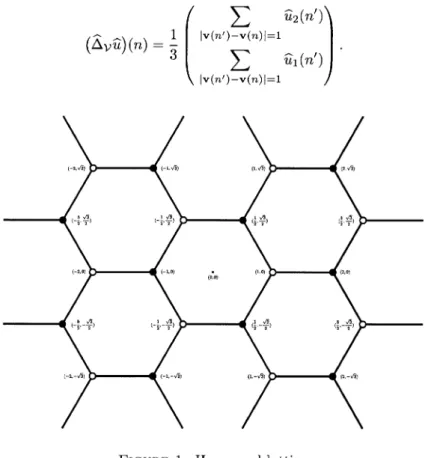
(2) 36 HIROSHI ISOZAKI. This is a joint work with K. Ando, E. Korotyaev and H. Morioka. 2. HEXAGONAL LATTICE AND ITS HAMILTONIAN. Figure 1 represents a hexagonal lattice.. We can find two lattices : the one. consisting of white dots, and the other black dots. Letting. \mathcal{L}_{0}=\{\mathrm{v}(n);n=(n_{1}, n_{2})\in \mathrm{Z}^{2}\}, \mathrm{v}(n)=n_{1}\mathrm{v}_{1}+n_{2}\mathrm{v}_{2},. \mathrm{v}_{1}=1+ $\omega$, \mathrm{v}_{2}= $\omega$(1+ $\omega$) , $\omega$=e^{ $\pi$ i/3}, we define the vertex set \mathcal{L}_{0} by. \mathcal{V}_{0}= (p_{1}+\mathcal{L}_{0})\cup(p_{2}+\mathcal{L}_{0}). .. Consequently, the wave function has two components in \ell^{2}(\mathrm{Z}) . Denoting it by û(n) (ûl (n) , û2 (n) ), we define the vertex Laplacian by =. ( $\Delta$\hat{}\mathcal{V} û)(n). =\displayst le\frac{1}3. \left(bgin{ary}l \sum_{| athrm{v}(n')-\mathr{v}(n)|=1\hat{u}_2(n')\ sum_{|\athrm{v}(n)-\mathr{v}(n)|=\mathr{l}\atu_{1}(n,) \ed{ary}\ight). FIGURE 1. Hexagonal lattice. To study the wave propagation on the lattice, let us first recall the case of continuous model, in which the free Schrödinger equation is. (-\triangle- $\lambda$)u=0..

(3) 37 INVERSE SCATTERING ON GRAPHEN. 1. 0 . The physical Passing to the Fourier transform, it becomes (| $\xi$|^{2}- $\lambda$)\overline{u}( $\xi$) L^{2} solution is the ‐density on the sphere, hence has the asymptotic expansion =. u(x)=C($\lambda$)\displaystyle\int_{S^{n-1} e^{i\sqrt{$\lambda$}$\omega$\cdotx}\overline{u}(\sqrt{$\lambda$}$\omega$)d$\omega$ \displaystyle\simeqC_{+}\frac{e^{i\sqrt{$\lambda$}r {r^(n-1)/2} (\sqrt{}$\lambda\theta$) \displaystle\frac{e^-i\sqrt{$\lambda$}r {^(n-1)/2} û. +C‐. û ( ‐ \sqrt{} $\lambda \theta$). with $\theta$=x/r, r= |x| . This also holds for the perturbed equation (-\triangle+V(x)$\lambda$)u=0 , where V(x) is compactly supported, i.e.. u(x)\displaystyle \simeq C_{+}\frac{e^{i\sqrt{$\lambda$}r }{r^{(n-1)/2} $\varphi$_{out}( $\theta$)+C_{-}\frac{e^{-i\sqrt{$\lambda$}r }{r^{(n-1)/2} $\varphi$_{in}( $\theta$) .. (2.1) The operator. S( $\lambda$):L^{2}(S^{n-1})\ni$\varphi$_{in}\rightarrow$\varphi$_{out}\in L^{2}(S^{n-1}) is the \mathrm{S} ‐matrix. Note that the sphere \sqrt{ $\lambda$}S^{n-1} is the characteristic surface of the operator -\triangle- $\lambda$.. The free Schrödinger equation on the hexagonal lattice is. (-\triangle_{\mathcal{V} - $\lambda$)\hat{u}=0\wedge. Passing to the Fourier series, we have. (H_{0}(x)- $\lambda$)u(x)=0 ,. on. \mathrm{T}^{2}=(\mathrm{R}/2 $\pi$ \mathrm{Z})^{2},. H_{0}(x)=-\displaystyle \frac{1}{3}\left(\begin{ar ay}{l l } & 0 & & 1+ & e^{-ix_{1} +e^{-ix_{2} \ 1+ & e^{ix_{1} & +e^{ix_{2} & & 0 \end{ar ay}\right).. The physical solution is an L^{2} ‐density supported in a submanifold on the torus:. M_{ $\lambda$}=\{x\in \mathrm{T}^{2};\det(H_{0}(x)- $\lambda$)=0\},. \displaystyle \det(H_{0}(x)- $\lambda$)=$\lambda$^{2}-\frac{1}{9}\{3+2(\cos x_{1}+\cos x_{2}+\cos(x_{1}-x_{2})\}. This is the characteristic surface of the difference operator the Fermi surface. The solution. u(x). -\triangle_{\mathcal{V} \wedge- $\lambda$ ,. and is called. is then written as. u(x)=\displaystyle \frac{ $\varphi$(x)}{p(x, $\lambda$)-i0}-\frac{ $\varphi$(x)}{p(x, $\lambda$)+i0}, $\varphi$(x)\in L^{2}(M_{ $\lambda$}) , p(x, $\lambda$)=\det(H_{0}(x)- $\lambda$). .. This also holds asymptotically (in the sense of singularity) for the perturbed lattice:. (2.2) and the operator. u(x)\displaystyle \simeq\frac{$\varphi$_{out}(x)}{p(x, $\lambda$)-i0}-\frac{$\varphi$_{in}(x)}{p(x, $\lambda$)+i0}, S( $\lambda$):L^{2}(M_{ $\lambda$})\ni$\varphi$_{in}\rightarrow$\varphi$_{out}\in L^{2}(M_{ $\lambda$}). is the \mathrm{S} ‐matrix.. The two terms appearing in the right‐hand side of (2.1) are called outgoing and incoming waves. As is seen here, they are distinguished by their spatial behaviors at 1_{\mathrm{I}\mathrm{n} this note, the Fourier trasnsform of a distribution u(x) on \mathrm{R}^{d} is denoted by \overline{u}( $\xi$) , while the Fourier coefficient of a distribution u(x) on the torus \mathrm{T}^{d} is denoted by û(n).

(4) 38 HIROSHI ISOZAKI. infimity. For the lattice, it does not work well, since the Fermi surface is in general not strictly convex and we encounter difficulties in applying the stationary phase method to the integral on it. Therefore, we pass to the Fourier series and observe the singularities of wave functions on the torus. This leads us to the formulation. (2.2). As a perturbation of the vertex model, we add a scalar potential, or (and) replace its finite part by a general graph. The associated Hamiltonian is denoted by \hat{H}_{\mathcal{V} . If these perturbations are assumed to be bounded self‐adjoint and confined in a compact part, the spectral theory can be developped easily.. We turn to the edge model, which is usually called the metric graph. We consider a hexagonal lattice with vertex set \mathcal{V} and edge set \mathcal{E} . Each edge \mathrm{e}\in \mathcal{E} is identified with the interval [0 , 1 ] . Functios on the edge set \mathcal{E} are denoted by \^{u}=\^{u} \mathcal{E} \{\hat{u}_{\mathrm{e} (z);\mathrm{e}\in \mathcal{E}\} . The Hamitonian \hat{H}_{\mathcal{E} is defined by =. (\displaystyle \hat{H}_{\mathcal{E} \hat{u}_{\mathcal{E} )_{\mathrm{e} (z)= (-\frac{d^{2} {dz^{2} +q_{\mathrm{e} (z) \hat{u}_{\mathrm{e} (z) , \mathrm{e}\in \mathcal{E}, assuming the Kirchhoff condition on û \mathcal{E} . For \mathrm{e} \in \mathrm{e}(0)=0, \mathrm{e}(1)=1 . Then, the Kirchhoff condition is. (K‐1) û \mathcal{E} (z) is continuous on. (K‐2) For each. \mathrm{e}\in \mathcal{E} ,. ûe. \in. \mathcal{E} ,. denote its end points by. \mathcal{E}.. C1 ([0,1. and. \displaystyle\sum_{\mathrm{e}(0)=v}\hat{u}_{\mathrm{e} '(0)=\sum_{\mathrm{e}(1)=v}\hat{u}_{\mathrm{e} '(1),\foral v\in\mathcal{V}. The assumption on the potentials are as follows:. (E‐1) q_{\mathrm{e} (z) is real‐valued, and q_{\mathrm{e}}(z)\in L^{2}(0,1) . (E‐2) q_{\mathrm{e}}(z)=0 except for a finite number of edges. (E‐3) q_{\mathrm{e}}(z)=q_{\mathrm{e}}(1-z) . This makes. \hat{H}_{\mathcal{E}. self‐adjoint on L^{2}(\mathcal{E}) .. There is a simple relation between the vertex Laplacian and the edge Laplacian. On each edge, the solution of the Schrödinger equation. (-(d/dz)^{2}+q_{\mathrm{e} (z)- $\lambda$)\hat{u}_{\mathrm{e} =\hat{f_{\mathrm{e} }. ,. on. (0,1). is written as. c_{\mathrm{e}(1, $\lambda$)\displayst le\frac{$\phi$_{\mathrm{e}0(z,$\lambda$)}{$\phi$_{\mathrm{e}0(1,$\lambda$)}+c_{\mathrm{e}(0, $\lambda$)\frac{$\phi$_{\mathrm{e}1(z,$\lambda$)}{$\phi$_{\mathrm{e}1(0,$\lambda$)}+r_{\mathrm{e}($\lambda$)\hat{f_\mathrm{e} , (d/dz)_{D}^{2}. where the equation. r_{\mathrm{e} ( $\lambda$)= (-(d/dz)_{D}^{2}+q_{\mathrm{e} (z)- $\lambda$)^{-1}. is the Dirichlet Laplacian on (0,1) , and $\phi$_{\mathrm{e}i}(z, $\lambda$) is the solution to. (-(d/dz)^{2}+q_{\mathrm{e} (z)- $\lambda$)$\phi$_{\mathrm{e}i}(z, $\lambda$)=0. ,. $\phi$_{\mathrm{e}0}(0, $\lambda$)=0, $\phi$_{\mathrm{e}0}'(0, $\lambda$)=1,. on. (0,1) ,.

(5) 39 INVERSE SCATTERING ON GRAPHEN. $\phi$_{\mathrm{e}\mathrm{i} (1, $\lambda$)=0, $\phi$_{\mathrm{e}1}'(1, $\lambda$)=-1. The coefficients c_{\mathrm{e} (1, $\lambda$) , c_{\mathrm{e} (0, $\lambda$) are determined by the Kirchhoff condition. The point is that. Kirchhoff condition. =. Vertex equation. Namely, the following equation holds:. \displayst le\sum_{\mathrm{e}(0)=v}\frac{1}$\phi$_{\mathrm{e}0(1,$\lambda$)}c_{\mathrm{e}(1, $\lambda$)+\sum_{\mathrm{e}(1)=v}\frac{1}$\phi$_{\mathrm{e}1(0,$\lambda$)}c_{\mathrm{e}(0, $\lambda$) +\displaystle\sum_{\mathrm{e}(0)=v}\frac{$\phi$_{\mathrm{e}1'(0,$\lambda$)}{ \phi$_{\mathrm{e}1(0,$\lambda$)}c_{\mathrm{e}(0, $\lambda$)-\sum_{\mathrm{e}(1)=v}\frac{$\phi$_{\mathrm{e}0'(1,$\lambda$)}{ \phi$_{\mathrm{e}0(1,$\lambda$)}c_{\mathrm{e}(1, $\lambda$) =\displaystyle\sum_{\mathrm{e}(1)=v}\frac{d} z}r_{\mathrm{e}($\lambda$)\hat{f_\mathrm{e} |_{z=1}-\sum_{\mathrm{e}(0)=v}\frac{d} z}r_{\mathrm{e}($\lambda$)\hat{f_\mathrm{e} |_{z=0}. Therefore, when q_{\mathrm{e}}(z)=0 , we have the following representation:. ( \displaystyle\hat{H}_{\mathcal{E}^{(0)}-$\lambda$)^{-1}\hat{f})|_{\mathrm{e}=c_{\mathrm{e}(1, $\lambda$)\frac{\sin\sqrt{$\lambda$}z{\sqrt{$\lambda$}+c_{\mathrm{e}(0, $\lambda$)\frac{\sin\sqrt{$\lambda$}(1-z)}{\sqrt{$\lambda$}+r_{\mathrm{e}^{(0)}($\lambda$)\hat{f_{\mathrm{e} , on each edge. \mathrm{e}. , and. c_{\mathrm{e} (1, $\lambda$)=c_{\mathrm{e}' (0, $\lambda$)= (\hat{R}_{\mathcal{V} ^{(0)}( $\lambda$)\hat{F}_{\mathcal{E} ^{(0)}( $\lambda$)\hat{f})(v). ,. for \mathrm{e}(1)=\mathrm{e}'(0)=v , where. \displaystyle\hat{R}_{\mathcal{V} ^{(0)}($\lambda$)=\frac{\sin\sqrt{$\lambda$} {\sqrt{$\lambda$} (-\trianglev\wedge+\cos\ qrt{$\lambda$})^{-1} (\hat{F}_{\mathcal{E} ^{(0)}( $\lambda$)\hat{f}) (v)=-\displaystyle \frac{1}{3}(\sum_{\mathrm{e}(1)=v}\frac{d}{dz}r_{\mathrm{e} ^{(0)}( $\lambda$)\hat{f_ \mathrm{e} |_{z=1}-\sum_{\mathrm{e}(0)=v}\frac{d}{dz}r_{\mathrm{e} ^{(0)}( $\lambda$)\hat{f_ \mathrm{e} |_{z=0}). .. This formula suggests that the properties of the continuous spectrum of the edge Schrödinger operator are inherited from those of the vertex Schrödinger operator. The spectra of the vertex and edge Schrödinger operators are as follows.. Lemma 2.1. (1) $\sigma$_{e}(\hat{H}_{\mathcal{V} )=[-1, 1]. (2) $\sigma$(\hat{H}_{\mathcal{E} )=[0, \infty)\cup$\sigma$_{D} , where $\sigma$_{D}=\displaystyle \bigcup_{\mathrm{e}\in \mathcal{E} $\sigma$_{p}(-(d/dz)_{D}^{2}+q_{\mathrm{e} (z) . 3. RELLICH TYPE THEOREM. To study the continuous model for the Schrödinger operator on. \mathrm{R}^{n} ,. appropriate. function spaces are the Besov type spaces B^{*}(\mathrm{R}^{n}) and B_{0}^{*}(\mathrm{R}^{n}) defined by. B^{*}(\displaystyle \mathrm{R}^{n})\ni f\Leftrightar ow\sup_{R>1}\frac{1}{R}\int_{|x|<R}|f(x)|^{2}dx<\infty, B_{0}^{*}(\displaystyle \mathrm{R}^{n})\ni f\Leftrightar ow\lim_{R\rightar ow\infty}\frac{1}{R}\int_{|x|<R}|f(x)|^{2}dx=0.. The following theorem, proven by Rellich and Bekua, is fundamental in studying the continuous spectrum..

(6) 40 HIROSHI ISOZAKI. Theorem 3.1. Let $\lambda$ > 0 . If u(x) \in B_{0}^{*}(\mathrm{R}^{n}) satisfies the Helmholtz equation (-\triangle- $\lambda$)u=0 on \{|x| >R\} for a constant R>0 , then u(x)=0 on \{|x| >R\}. This theorem implies the non‐existence of eigenvalues embedded in the continu‐ ous spectrum. It also palys an important role in the inverse scattering theory.. We consider the counter part of this theorem on the lattice. For the periodic lattice \mathcal{V} , we define the Besov type speces by. B^{*}(\displaystyle \mathcal{V})\ni\hat{v}\Leftrightar ow\sup_{R>1}\frac{1}{R}\sum_{|n<R}|\hat{v}(n)|^{2}<\infty, B_{0}^{*}(\displaystyle \mathcal{V})\ni\hat{v}\Leftrightar ow\lim_{R\rightar ow\infty}\frac{1}{R}\sum_{|n<R}|\hat{v}(n)|^{2}=0.. Passing to the Fourier series, we define. B^{*}(\mathrm{T}^{d})\ni v\Leftrightarrow\hat{v}\in B^{*}(\mathcal{V}). B_{0}^{*}(\mathrm{T}^{d})\ni v\Leftrightarrow\hat{v}\in B_{0}^{*}(\mathcal{V}). ,. .. Sometimes, it is more convenient to use the Fourier transform. Multiplying a cut‐. off function (a partition of unity) and passing to the Fourier transform \overline{v}( $\xi$) , we can also define. B^{*}(\displaystyle \mathrm{T}^{d})\ni v\Leftrightar ow\sup_{R>1}\frac{1}{R}\int_{|x<R}|\overline{v}( $\xi$)|^{2}d $\xi$<\infty, B_{0}^{*}(\displaystyle \mathrm{T}^{d})\ni v\Leftrightar ow\lim_{R\rightar ow\infty}\frac{1}{R}\int_{|x<R}|\overline{v}( $\xi$)|^{2}d $\xi$=0.. For the lattice space, the Rellich type theorem should be rephrased as follows.. Theorem 3.2. Suppose \^{u}\in B_{0}^{*}(\mathcal{V}) satisfies lattice space. Then, \hat{v}=0 near infinity.. Extending û to be. 0. (-\hat{ $\Delta$}_{\mathcal{V} - $\lambda$)\hat{v}=0. near infinity of the. in the finite part and passing to the Fourier series, we obtain. the equation. (H_{0}(x)- $\lambda$)u(x)=f(x). ,. where f(x) is a trigonometric polynomial, since its Fourier coefficients are compactly supported. Then, the Rellich type theorem on the lattice is formulated and proved in the following form.. Theorem 3.3. Let $\lambda$\in(-1,1)\backslash \{0, \pm 1/3, \pm 1\} . Let u(x) \in B_{0}^{*}(\mathrm{T}^{2}) satisfy (H_{0}(x)$\lambda$)u(x) f(x) , where f(x) is a trigonometric polynomial. Then, u(x) is also a =. trigonometric polynomial.. The proof relies on the HilbertNullStellenSatz ([18], [2]). Similar theorem also holds for the edge Hamiltonian. In particular, the non‐existnece of embedded eigen‐ values follows. Put. $\sigma$_{\mathcal{V}}=(-1,1)\backslash \{0, \pm 1/3, \pm 1\},. $\sigma$_{\mathcal{E} =(0, \infty)\backslash ($\sigma$_{D}\cup\{ $\lambda$;-\cos\sqrt{ $\lambda$}=0, \pm 1/3, \pm 1\}). ..

(7) 41 INVERSE SCATTERING ON GRAPHEN. Corollary 3.4. (1) $\sigma$_{p}(\hat{H}_{\mathcal{V} )\cap$\sigma$_{\mathcal{E} =\emptyset. (2) $\sigma$_{p}(\hat{H}_{\mathcal{E} )\cap$\sigma$_{\mathcal{E} =\emptyset. For the preceeding results about the spectra of vertex models and edge models,. see e.g. [6], [16], [14], [5], [6], [13]. 4. FORWARD PROBLEM. For the vertex model, the space. \hat{B}(\mathcal{V}). is defined by. \displaystyle \hat{B}(\mathcal{V})\ni\hat{f}\Leftrightar ow\sum_{j=0}^{\infty}r_{j}^{1/2}(\sum_{r_{j-1}\leq|n<r_{j} |\hat{f}(n)|^{2})^{1/2}<\infty, where space. r_{-1}. =. 0, r_{j}. =. 2^{j}. (j \geq 0) .. \hat{B}(\mathcal{V}) , \hat{B}^{*}(\mathcal{V}). Then, the spaces. rig the Hilbert. \ell^{2}(\mathcal{V}) :. \hat{B}(\mathcal{V}) \subset\ell^{2}(\mathcal{V})\subset\hat{B}^{*}(\mathcal{V}) For the edge model, the Besov type spaces \hat{B}(\mathcal{E}) , \hat{B}^{*}(\mathcal{E}) , \hat{B}_{0}^{*}(\mathcal{E}) are defined similarly, .. \mathrm{e}.\mathrm{g}.. \displaystyle\hat{B}^{*}(\mathcal{E})\ni\hat{f}\Leftrightar ow\sup_{R>1}\frac{1}{R}\sum_{\mathrm{e}\subsetB_{R}\Vert\hat{f_{\mathrm{e} \Vert_{L^{2}(0,1)}^{2}<\infty,. where B_{R}=\{x\in \mathrm{R}^{2}; |x| <R\} . Their counter parts on the torus are defined by. B(\mathrm{T}^{2}\times I_{\mathcal{E} )\ni f\Leftrightar ow\hat{f}\in\hat{B}(\mathcal{E}) B^{*}(\mathrm{T}^{2}\times I_{\mathcal{E} )\ni f\Leftrightar ow\hat{f}\in\hat{B}^{*}(\mathcal{E}) B_{0}^{*}(\mathrm{T}^{2}\times I_{\mathcal{E} )\ni f\Leftrightar ow\hat{f}\in\hat{B}_{0}^{*}(\mathcal{E}) ,. where I_{\mathcal{E} =(0,1) , and. \hat{f} denotes the. *. ,. Fourier coefficient of f(x, z) with respect to. (with a suitable cut‐off function). (\hat{H}_{\mathcal{V} -z)^{-1} and \hat{R}_{\mathcal{E} (z) Let \hat{R}_{\mathcal{V} (z) =. ,. =. (\hat{H}_{\mathcal{E} -z)^{-1} .. x. Then, the following weak. ‐limits exist.. Theorem 4.1. For $\lambda$\in$\sigma$_{\mathcal{V} ,. \hat{R}_{\mathcal{V} ( $\lambda$\pm i0)\in \mathrm{B}(\hat{B}(\mathcal{V});\hat{B}^{*}(\mathcal{V}) .. Theorem 4.2. For. \hat{R}_{\mathcal{E} ( $\lambda$\pm i0) \in \mathrm{B}(\hat{B}(\mathcal{E});\hat{B}^{*}(\mathcal{E}) .. $\lambda$\in$\sigma$_{\mathcal{E} ,. Once we have proven this limiting absorption principle, one can follow the sta‐. tionary theory of scattering developed by Kato‐Kuroda [12], Ikebe [10], Agmon [1] without any difficulty, namely, existence and completeness of time‐dependent wave operators, eigenfunction expansion theory, unitarity of the representation by generalized eigenfunctions.. \mathrm{S} ‐matrix. and its. In some energy region, one can define the \mathrm{S} ‐matrix by using the asymptotic behavior of wave functions at the infinity of the lattice space. However, for both of the vertex model and the edge model, it is more convenient to obeserve the behavior of singularities of wave functions on the torus, since there is no restricton of energy. For the vertex model, it is stated as follows. Recall that H_{0}(x) has two eigenvalues. $\lambda$_{j}(x) and the eigenprojections P_{j}(x) , j=1 , 2. Define. M_{ $\lambda$,j}=\{x\in \mathrm{T}^{2};$\lambda$_{j}(x)= $\lambda$\},.

(8) 42 HIROSHI ISOZAKI. M_{ $\lambda$}=M_{ $\lambda$,1}\cup M_{ $\lambda$,2}. Theorem 4.3. Let. L^{2}(M_{ $\lambda$}) and û. \in. $\lambda$ \in $\sigma$_{\mathcal{V} .. For any $\varphi$^{in}. \in. L^{2}(M_{ $\lambda$}) , there exist a unique $\varphi$^{out}. \in. *. B ( \mathcal{V} ) such that. (\hat{H}_{\mathcal{V} - $\lambda$)\hat{u}=0,. u\displaystyle \simeq\frac{1}{2 $\pi$ i}\sum_{j=1,2}\frac{1}{$\lambda$_{j}(x)- $\lambda$\mp i0}\otimes P_{j}(x)$\varphi$^{out} -\displaystyle \frac{1}{2 $\pi$ i}\sum_{j=1,2}\frac{1}{$\lambda$_{j}(x)+ $\lambda$\mp i0}\otimes P_{j}(x)$\varphi$^{in},. where f\simeq g means f-g\in B_{0}^{*}(\mathrm{T}^{2}) . The unitary operator. S( $\lambda$):L^{2}(M_{ $\lambda$})\ni$\varphi$^{in}\rightarrow$\varphi$^{out}\in L^{2}(M_{ $\lambda$}) is the S‐matrix.. For the edge model, the above theorem is stated as follows.. Theorem 4.4. Let $\lambda$\in$\sigma$_{\mathcal{E} . For any incoimg data. a unique solution û. \in. \hat{}*. B. ( \mathcal{E} ). $\phi$^{in}\in L^{2}(M_{-\cos\sqrt{ $\lambda$}}) ,. there exist. of the equation. (\hat{H}_{\mathcal{E} - $\lambda$)\hat{u}=0, and an outgoing data. $\varphi$^{out}\in L^{2}(M_{-\cos\sqrt{ $\lambda$}}). satisfying. u\displaystyle \simeq B( $\lambda$)\sum_{j=1,2}\frac{1}{$\lambda$_{j}(x)+\cos\sqrt{ $\lambda$}-i $\epsilon$( $\lambda$)}\otimes P_{j}(x)$\varphi$^{out} -B( $\lambda$)\displaystyle \sum_{j=1,2}\frac{1}{$\lambda$_{j}(x)+\cos\sqrt{ $\lambda$}+i $\epsilon$( $\lambda$)}\otimes P_{j}(x)$\varphi$^{in},. where f\simeq g means f-g\in B_{0}^{*} (\mathrm{T}^{2} \times I_{\mathcal{E} ) . The unitary operator. S( $\lambda$):L^{2}(M_{-\cos\sqrt{ $\lambda$}}) \in$\varphi$^{in}\rightarrow$\varphi$^{out}\in L^{2}(M_{-\cos\sqrt{ $\lambda$}}) is the S‐matrix.. Here B( $\lambda$) \in \mathrm{B}(B^{*}(\mathrm{T}^{2}\times I_{\mathcal{E} );B^{*}(\mathrm{T}^{2}\times I_{\mathcal{E} ) and $\epsilon$( $\lambda$)=\pm 1 , however we omit the precise definition. 5. FROM. \mathrm{S} ‐MATRIX. TO D‐N MAP. As in the case of continuous model, the inverse scattering on the whole space is reduced to an inverse boundary value problem in a bounded domain. Take a. sufficiently large bounded set containing all perturbations. Then, the equation in the whole space is split into three parts: the exterior boundary value problem, the. interior boundary value problem and the (integral) equation on the boundary. We follow the same approach for the vertex model and edge model. Take a bounded domain $\Omega$_{int} enclosing all perturbations, and let $\Omega$_{ext} be the exterior do‐ main so that. $\Omega$_{ext}\cup$\Omega$_{int}=\mathcal{V}, \partial$\Omega$_{\mathrm{e}xt}=\partial$\Omega$_{int}..

(9) 43 INVERSE SCATTERING ON GRAPHEN. Consider the Dirichlet problem. \left{\begin{ar y}{l (-\hat{$\Delta$}_{\mathcl{V}-$\lambda$)\hat{u}=0,\mathrm{i}\mathrm{n}$\Omega$_{int},\ ^{u}=f\hat{},\mathrm{o}\mathrm{n}\partil$\Omega$_{int}. \end{ar y}\right. The Neumann derivative is defined by. \partial_{\mathrm{v} \hat{u}=-\hat{$\Delta$}_{\mathcal{V} \hat{u}|_{\partial$\Omega$_{int} Then, the D‐N map, Dirichlet‐to‐Neumam map, is defined by. $\Lambda$_{int}( $\lambda$):\hat{f}\rightar ow\partial_{ $\nu$}\hat{u}. The \mathrm{S} ‐matrix is defined in the whole space and in the exterior domain as well. We. denote them S( $\lambda$) and S_{ext}( $\lambda$) , and define the scattering amplitudes. S( $\lambda$)=I-2 $\pi$ iA( $\lambda$) , S_{ext}( $\lambda$)=I-2 $\pi$ iA_{ext}( $\lambda$). .. Then, the following formula holds:. (5.1). A_{ext}( $\lambda$). — A ( $\lambda$ ). =. î( + ) ( $\lambda$)B_{ $\Sigma$}( $\lambda$)^{-1}(\hat{I}^{(-)}( $\lambda$))^{*},. B_{ $\Sigma$}( $\lambda$)=$\Lambda$_{int}( $\lambda$)-$\Lambda$_{ext}( $\lambda$)- $\lambda \chi \Sigma$.. Here,. $\Sigma$=\partial$\Omega$_{int}=\partial$\Omega$_{ext} ,. î( \pm ) ( $\lambda$ ) : L^{2}(M_{ $\lambda$})\rightarrow l^{2}( $\Sigma$) are some injective operators,. $\Lambda$_{ext}( $\lambda$) is the D‐N map in the exterior domain, and. of $\Sigma$ . Since all perturbations are confined to. x $\Sigma$. $\Omega$_{int} ,. is the characterisitic function. we know î (\pm)( $\lambda$) and $\Lambda$_{ext}( $\lambda$) .. Therefore, (5.1) means that S( $\lambda$) and $\Lambda$_{int}( $\lambda$) determine each other. The edge model can be dealt with similarly.. 6. INVERSE SCATTERING. 6.1. Vertex model‐ reconstruction of the potential. In the inverse boundary value problem for the continuous case, the exponentially growing solution for the Schrödinger equation plays an important role. It solves the Schrödinger equation. (-\triangle+V(x)- $\lambda$)u. =0. in. \mathrm{R}^{n} ,. and is exponentially growing in a half‐space, and. exponentially decaying in the opposite half‐space. There is a counter part of this. solution in the discrete model. In [11], we used a solution to the discrete Schrödinger equation on the square lattice, which vanishes in a half‐space and non‐zero in the opposite half‐space, to recontsruct the scalar potential from the \mathrm{S} ‐matrix. A similar idea works well for the hexaogonal lattice.. Theorem 6.1. Consider the vertex Schrödinger operator on the hexagonal lattice with a compactly supported scalar potential. Then, the potential is uniquely recon‐ structed from the S‐matrix S( $\lambda$) for an arbitrarily given fixed energy $\lambda$\in$\sigma$_{\mathcal{V} ..

(10) 44 HIROSHI ISOZAKI. 6.2. Vertex model‐recovery as a planar graph. Another central issue in the inverse boundary value problem for the continuous model is the reconstruction of. the Riemannian metric from the D‐N map with 0 energy. This is an interpretation of the inverse problem of electrical impedance tomography. We expect that the metric is determined by the D‐N map up to a diffeomorphism which leaves the boundary of the domain invariant. It is proved in 2‐dimensions in the general setting, and for the real analytic case with dimension n\geq 3. The counter part of the Riemannian manifold in the discrete model is the planar. graph. By the works of Colin de Verdière [7], [8] and Curtis‐Morrow [9], it is known that the D‐N map determines the planar graph up to elementary transformations. In the case of hexagonal lattice, the D‐N map for the planar graph corresponds to the \mathrm{S} ‐matrix with energy at the bottom of the continuous spectrum. Therefore, we obtain the following theorem.. Theorem 6.2. For a sequence of energies $\lambda$_{n}. \in $\sigma$_{\mathcal{V}. such that $\lambda$_{n}. \rightarrow. -1 ,. the S‐. matrices S($\lambda$_{n}) determine the perturbed finite part of the hexagonal lattice up to elementary transformations.. The equivalence of the \mathrm{S} ‐matrix and the D‐N map can be proven for a wide class. of lattices, e.g. those introduced in [2]. Therefore, Theorem 6.2 holds for such class of vertex models.. 6.3. Vertex model ‐ proving defects. A physically important example of the perturbation as a graph is the defect of the lattice. We consider the case where the. defects are bounded. By virtue of Theorem 6.2, one can reconstruct the perturbed graph topologically. However, it does not give the information of the location of defects. To study it, we utilize the above mentioned analogue of exponentially growing solution to the Schrödinger equation on the hexagonal lattice. Take a straight line L in the lattice and construct the solution to the free Schrödinger equation which vanishes below L but does not vanish above L . Suppose that the all defects are lying below L . If we take it as an input of the D‐N map, the output is the same as that of the unperturbed case. Let us move the line L downwards. Then, it will touch the defects. At this moment, the output of the D‐N map changes, and we conclude that there is a defect on the line L . Therefore, we can enclose the. defects from above. Changing the dierction of the line. L,. we get the following. theorem.. Theorem 6.3. Assume that the defects consist of finite convex polygons. Then, from the S‐matrix S( $\lambda$) with an arbitrarily fixed energy $\lambda$\in$\sigma$_{\mathcal{V} , one can determine the convex hull of the defects.. Theorems 6.1 ,6.2, 6.3 will appear in [3]. 6.4. Edge model‐ reconstuction of the potential. One can use the same idea. for the edge model. By the above procedure, one can compute the coefficients for the.

(11) 45 INVERSE SCATTERING ON GRAPHEN. perturbed vertex Laplacian from the D‐N map. It consists of $\phi$_{\mathrm{e}0}(0, $\lambda$) , where $\phi$_{\mathrm{e}0}(z) is the solution to the Schrödinger equation (-(d/dz)^{2}+q_{\mathrm{e}}(z)- $\lambda$)$\phi$_{\mathrm{e}0}(z, $\lambda$)=0 with. initial data $\phi$_{\mathrm{e}0}(0, $\lambda$)=0 . Then, the zeros of $\phi$_{\mathrm{e}(0)}(0, $\lambda$) are the Dirichlet eigenvalues of the operator -(d/dz)^{2}+q_{\mathrm{e}}(z)- $\lambda$ . Recall Borg’s theorem [4], which is the starting point of the inverse spectral theory: A symmetric potential on (0,1) is determined by its Dirichlet eigenvalues. We have thus arrived at the following theorem. Theorem 6.4. Let I be an open interval in $\sigma$_{\mathcal{E} . Then, the potential is determined from the S‐matrix S( $\lambda$) for all energies $\lambda$\in I.. One can also deal with non‐zero back ground potentials.. Theorem 6.5. Let q_{0}(z) \in L^{2}(0,1) be real and symmetric. Suppose that the edge potentials q_{\mathrm{e} (z) coincide with q_{0}(z) except for a finite number of edges. Let I be an open interval in $\sigma$_{\mathcal{E} . Then, the potential q_{\mathcal{E} is determined from the S‐matrix S( $\lambda$) for all energies $\lambda$\in I. REFERENCES. [1] S. Agmon and L. Hörmander, Asymptotic properties of solutions of differential equations with simple characteristics, J. d’Anal. Math., 30 (1976), 1‐38. [2] K. Ando, H. Isozaki and H. Morioka, Spectral properties of Schrödinger operators on perturbed lattices, Ann. Henri Poincaré 17 (2016), 2103‐2171. [3] K. Ando, H. Isozaki and H. Morioka, Inverse scattemng for Schrödinger operators on per‐ turbed lattices, in preparation.. [4] G. Borg, Eine Umkehrung der Sturm‐Liouvilleschen Eigenwertaufgabe. Bestimmung der Dif‐ ferentialgleichung durch die Eigenwerte, Acta Math. 78 (1946), 1‐96. [5] J. Brüning, V. Geyley and K. Pankrashkin, Spectra of self‐adjoint extensions and applications to solvable Schrödînger operators, Rev. Math. Phys. 20 (2008), 1‐70. [6] C. Cattaneo, The spectrum of the continuous Laplacian on a graph, Monatsh. Math. 124 (1997), 215‐235. [7] Y. Colin de Verdière, Réseaux électriques planaires I, Commentarii Math. Helv., 69 (1994), 351‐374.. [8] Y. Colin de Verdière, I. de Gitler and D. Vertigan, Réseaux électriques planaires II, Com‐ mentarii Math. Helv., 71 (1996), 144‐167. [9] E. B. Curtis and J. A. Morrow, Inverse Problems for Electrical Networks, World Scientific, Singapore‐New Jersey‐London‐Hong Kong (2000). [10] T. Ikebe, Eigenfunction expansions associated with the Schrödinger operators and their ap‐ plications to scattering theory, Arch. Rational Mech. Anal. 5 (1960), 1‐34. [11] H. Isozaki and H. Morioka, Inverse scattering at a fixed energy for discrete Schrödinger operators on the square lattice, Ann. l’Inst. Fourier 65 (2015), 1153‐1200. [12] T. Kato and S. T. Kuroda, Theory of simple scattering and eigenfunction expansions, Funct. Anal. and Related Fields (F. $\Gamma$ . Browder, ed Springer, Berlin, Heideberg, Nee York (1970), 99‐131.. [13] E. Korotyaev and N. Saburova, Scattering on metmc graphs, arXiv:1507. 06441vl [math.SP] 23 Jul 2015.. [14] P. Kuchment and O. Post, On the spectra of carbon nano‐structures, Commun. Math. Phys. 275 (2007), 805‐826. [15] P. Kuchment and B. Vainberg, On absence of embedded eigenvalues for Schrödinger operators with perturbed periodic potentials, Comm. PDE, 25 (2000), 1809‐1826. [16] K. Pankrashkin, Spectra of Schrödinger operators on equilateral quantum graphs, Lett. Math. Phys. 77 (2006), 139‐154. [17] J. Pöschel and E. Trubowitz, Inverse Spectral Theory, Academic Press, Boston, (1987). [1S] W. Shaban and B. Vainberg, Radiation conditions for the difference Schrödinger operators, Applicable Analysis, 80 (2001), 525‐556..

(12) 46 HIROSHI ISOZAKI. PROFESSOR EMERITUS, UNIVERSITY OF TSUKUBA, TSUKUBA, 305‐8571, JAPAN.

(13)