Solvable models in the scattering theory for the Aharonov-Bohm effect (Tosio Kato Centennial Conference)

全文

(1)68. 数理解析研究所講究録第2074巻 2018年 68-79. Solvable models in the scattering theory for the Aharonov‐Bohm effect Takuya MINE (Kyoto Institute of Technology) Abstract. We briefly review the scattering theory for the Schrödinger operator related to the Aharonov‐ Bohm effect, by exhibiting some explicitly solvable models; an infinitesimally thin solenoid in \mathbb{R}^{2}, two infinitesimally thin solenoids with the quantized magnetic fluxes in \mathbb{R}^{2} , and an infinitesimally thin ring solenoid with the quantized magnetic flux in \mathbb{R}^{3} . We give explicit formulas for the incoming wave solution and the scattering amplitude for these models in terms of some special functions, with the graphs obtained by a numerical method. We also review known high‐energy asymptotic formulas related to these examples.. 1. Introduction. In 1959, Y. Aharonov and D. Bohm published a remarkable paper [Ah‐Bo], in which they stated that the magnetic field enclosed in an electrically shielded solenoid can affect the electron moving outside the solenoid through the magnetic vector potential, in the formulation of non‐relativistic quantum mechanics. This phenomenon is called the Aharonov‐Bohm effect, and there was a large controversy. concerning the existence of the Aharonov‐Bohm effect in the real world (for the detail, see e.g. Peshkin‐ Tonomura [Pe‐To]). The decisive experiment was done by A. Tonomura et al. [To]. They prepared toroidal apparatus in which they succeeded to enclose the magnetic field completely with the aid of the super‐conductive effect, and observed the interference pattern by two coherent electron beams going through inside and outside the hole of the toroidal magnet. The obtained picture clearly shows that the. phase shift of the electron wave by the magnetic flux inside the torus1.. There are also numerous works concerning the direct and the inverse scattering theory related to the Aharonov‐Bohm effect. First, we list the results about the Schrödinger operator H_{N} in \mathbb{R}^{2} with N. pointlike magnetic fields (for the definition of H_{N} , see (5) below), which models. infinitesimally thin solenoids perpendicular to the plane. The case. N=1. N. infinitely long,. is studied by Aharonov‐Bohm. [Ah‐Bo], and later more mathematically rigorously by Ruijsenaars [Ru]. In the case. , Št ovíček \check{}. N \geq 2. [St] constructs the Green function of H_{2} by path‐integral method, and the result is further developed. in Kocábová‐Štovíček [Ko‐Stl] and Koštáková‐Štovíček [Ko‐St2]. Nambu [Na] tries to calculate the. scattering amplitude for H_{N} , but it is not successful (instead, Nambu studies the dynamical vortices). Ito‐Tamura [It‐Tal, It‐Ta2] obtain the asymptotic formula for the scattering amplitude for H_{N} , in the limit the distance between solenoids tends to infinity. Roux‐Yafaev [Ro‐Ya] study the essential spectrum of the scattering matrix for more general magnetic Schrödinger operator in \mathbb{R}^{2} , including the. Aharonov‐Bohm one. Yafaev [Ya] also studies the diagonal singularity of the scattering amplitude for the magnetic Schrödinger operators in \mathbb{R}^{d} (d=2,3) . There are a lot of results about the inverse scattering problem for H_{N} or related magnetic Schrödinger. operators in \mathbb{R}^{d} (d \geq 2) ; e.g. Arians [Ar] (d \geq 2) , Nicoleau [Ni] (d \geq 2) , Weder [We] (d = 2) , Es‐ kin [Esl, Es2] (d \geq 2) , Ballesteros‐Weder [Ba‐Wel, Ba‐We2, Ba‐We3] (d = 3) , and Eskin‐Isozaki‐ O’Dell [Es‐Is‐Od] (d=2) (for more comprehensive list, see Eskin [Es3]). Especially, Ballesteros‐Weder [Ba‐Wel, Ba‐We2, Ba‐We3] give a detailed analysis of the scattering by toroidal magnetic fields in \mathbb{R}^{3} , and the result in [Ba‐We2] is considered to be a mathematical justification of the experiment by Tonomura et al. [To]. We also note that Iwatsuka−M−Shimada [Iw‐Mi‐Sh] prove the norm‐resolvent 1The picture can also bc sccn in Hitachi’s web‐site. http: //\mathrm{v}m\mathrm{w} . hitachi. com/rd/portal/highlight/quant \mathrm{u}\mathrm{m}/\mathrm{a}\mathrm{h}\mathrm{a}\mathrm{r}\mathrm{o}\mathrm{n}\mathrm{o}\mathrm{v}-\mathrm{b}\mathrm{o}\mathrm{h}\mathrm{m}/ index. html.

(2) 69. convergence of the Schrödinger operators with toroidal magnetic fields in the limit as the thickness of the torus tends to 0 with fixed magnetic flux through the section of the torus.. However, the paper by Gu‐Qian [Gu‐Qi] seems to be missed in the previous papers. Gu‐Qian. calculate the scattering amplitude for the Schrödinger operator H_{2} in \mathbb{R}^{2} with two pointlike magnetic fields, by using the elliptic coordinate. The result of Gu‐Qian is mathematically not complete, and. the author justifies Gu‐Qian’s result in [Mil, Mi2] under the magnetic quantization condition (see (7) below), that is, the magnetic flux of each pointlike field is an integer multiple of the quantum of magnetic flux. The condition (7) comes from the covering structure of the elliptic coordinate as a map from \mathbb{R}^{2} onto itself (see [Mil]). Interestingly, the condition (7) matches with the experiment by Tonomura et al. [To] (the magnetic flux is quantized by a super‐conductive effect), and also plays an important role in the nodal domain problem for the Schrödinger operators with AB‐magnetic fields (see Helffer [He] and references therein). In this short note, we exhibit some explicitly solvable models, in the sense that we can calculate the incoming plane wave and the scattering amplitude explicitly in terms of some special functions. We also give the graphs obtained by a numerical method, which help an intuitive understanding of the Aharonov‐Bohm effect. In sections 2 and 3, we study the Schrödinger operator with N pointlike magnetic fields in \mathbb{R}^{2} , which models N infinitely long, infinitesimally thin solenoids perpendicular to 1 ([Ah‐Bo, Ru]; see also Theorem the plane. It is well‐known that the model is solvable when N 2 , the model is solvable in the elliptic coordinate, if the magnetic fluxes are 2.1 below). When N quantized to be integer multiples of the quantum of magnetic flux ([Gu‐Qi, Mil, Mi2]; see also Theorem 3.2 below). We also review the asymptotic formula of the scattering amplitude by Ito‐Tamura [It‐Tal], =. =. and compare their result with the explicit formula. In section 4, we consider the Schrödinger operator with a toroidal magnetic field in \mathbb{R}^{3} , which models the experiment by Tonomura et al., especially we. review the result by Ballesteros‐Weder [Ba‐We2]. In the limiting case the torus becomes a ring of thickness 0 . and the flux through the section of the ring is quantized to be an integer multiple of the quantum of magnetic flux, the model is solvable in the oblate spheroidal coordinate (Theorem 4.1). The. last result seems to be new (there is no proof here, and the proof will be written elsewhere). All the figures except Figure 7 are obtained by using Wolfram Mathematica 10.3.. Scattering by single solenoid in \mathbb{R}^{2}. 2. In the paper Aharonov‐Bohm [Ah‐Bo], they study the scattering of an electron by an infinitesimally. thin, infinitely long magnetic solenoid, parallel to the. z. ‐axis. Because of the translational invariance. along the z ‐axis, they consider the two‐dimensional Hamiltonian2 H=. (\displaystyle\frac{1}{i \nabla-A_{$\alpha$})^{2}. on. \mathbb{R}^{2},. \nabla=. (\displayst le\frac{\parti l}{\parti lx'}\frac{\parti l}{\parti ly}). A_{ $\alpha$}=(A_{ $\alpha$,x}, A_{ $\alpha$,y})= $\alpha$(-\displaystyle \frac{y}{r^{2} , \frac{x}{r^{2} ) , r=\sqrt{x^{2}+y^{2} ,. (1). with the regular boundary condition at (x, y) =O= (0,0) (we use the normalization \hslash=1, m= 1/2, 1 for simplicity). and e Here $\alpha$ is a real constant, and the z‐component of the magnetic field =. corresponding to the magnetic vector potential A_{ $\alpha$} is given by curl. A_{$\alpha$}=\displaystyle\frac{\partialA_{$\alpha$,y} {\partialx}-\frac{\partialA_{$\alpha$,x} {\partialy}=2$\pi\alpha\delta$_{O},. where $\delta$_{O} is the Dirac measure at the origin. Aharonov and Bohm compute the incoming wave solution $\varphi$- =$\varphi$_{-}(\mathrm{x};\mathrm{p}) to the stationary Schrödinger equation H$\varphi$_{-} =k^{2}$\varphi$_{-} (k>0) , which behaves like. '. $\varphi$_{-}(\displaystyle \mathrm{x};\mathrm{p}) \sim e^{i\mathrm{x}\cdot \mathrm{p} +f( $\tau$\rightar ow $\theta$;k^{2})\frac{e^{ikr} {r^{1/2} (r\rightar ow\infty). ,. Here the sign of is oppositc to the one used in Aharonov‐Bohm [Ah‐Bo] and Ruijsenaars [Ru], rather our choice matches with the one in Ito‐Tamura [It‐Tal]. So the formula (3) does not seem to coincide with [Ru, (4.11)], but it coincides with [It‐Tal, (1.2)]. $\alpha$.

(3) 70. where. \mathrm{x}=. (x, y). =. (rcos $\theta$, r sine), and. \mathrm{p}. =. (kcos $\tau$ , ksin $\tau$ ) is the momentum of the incident wave3.. The factor f( $\tau$\rightarrow $\theta$;k^{2}) is called the scattering amplitude, and |f( $\tau$\rightarrow $\theta$;k^{2})|^{2} the differential scattering cross section, which tells us the ratio of the particles coming from the incident direction $\tau$ and scattered. into the final direction $\theta$.. Ruijsenaars [Ru] studies this problem mathematically more rigorous way. Especially Ruijsenaars proves that the incoming wave solution $\varphi$_{-} is also defined as the integral kernel of the wave operator W_{-} in the time‐dependent formalism, as follows.. =\displaystyle \mathrm{s}-\lim_{t\rightar ow-\infty}e^{itH}e^{-itH_{0}. W_{-}u(\displaystyle\mathrm{x})=\frac{1}{2$\pi$}\int_{\mathb {R}^{2} $\varphi$_{-} (. \mathrm{x}. ; \mathrm{p} )û (\mathrm{p})d\mathrm{p} ,. (2). where \displaystyle \^{u}(\mathrm{p})=(2 $\pi$)^{-1}\int_{\mathbb{R}^{2} e^{-i\mathrm{x}\cdot \mathrm{p} u(\mathrm{x})d\mathrm{x} is the Fourier transform of u . Since the expression (2) is obtained by replacing e^{i\mathrm{x}\cdot \mathrm{p} in the Fourier inversion formula by $\varphi$_{-}(\mathrm{x};\mathrm{p}) , we sometimes use the formal expression W_{-}e^{i\mathrm{x}\cdot \mathrm{p} . Ruijsenaars also calculates the singularity of the scattering amplitude at the $\varphi$-(\mathrm{x};\mathrm{p}) =. forward direction $\tau$= $\theta$ . Their results are summarized as follows.. Theorem 2.1 (Aharonov‐Bohm [Ah‐Bo], Ruijsenaars [Ru]). Put \mathrm{x}=(x, y)= ( r\cos $\theta$ , rsin $\theta$ ), and ( k\cos $\tau$ , ksin $\tau$ ). Then, the following holds.. \mathrm{p}=. (i) The incoming wave solution. $\varphi$_{-}. is given by. $\varphi$_{-}(\displaystyle\mathrm{x};\mathrm{p})=\sum_{m=-\infty}^{\infty}i^{|m|}e^{i$\delta$_{\upar own,k} J_{|m-\mathrm{a}| (kr)e^{im($\theta$-$\tau$)}, where J_{ $\nu$} is the Bessel function of order v , and $\delta$_{m_{i}k}=(|m|-|m- $\alpha$|) $\pi$/2.. (ii) The scattering amplitude f( $\tau$\rightarrow $\theta$;k^{2}) is given by. f( $\tau$\rightarrow $\theta$;k^{2}) =. (\displaystyle\frac{2$\pi$}{ik})^{1/2} ( (\displaystyle\cos$\alpha\pi$-1)$\delta$($\theta$-$\tau$)-\frac{i\sin$\alpha\pi$}{$\pi$}e^{i[$\alpha$]($\theta$-$\tau$)} . . \displaystle\frac{e^i($\thea$- \tau$)}{e^i($\thea$- \tau$)}-1 ), \mathrm{P} \mathrm{V}. (3). where [x] is the integer part ofx and P.V. denotes the principal value. In particular, the differential scattering cross section |f( $\tau$\rightarrow $\theta$;k^{2})|^{2} is given by. |f($\tau$\displaystyle\rightar ow$\theta$;k^{2})|^{2}=\frac{1}{2$\pi$k}\frac{\sin^{2}($\alpha\pi$)}{\sin^{2}( $\theta$-$\tau$)/2)}($\theta$\neq$\tau$). .. The number $\delta$_{m,k} is called the scattemng phase shift, which is determined by the asymptotic formula. J_{|m- $\alpha$|}(kr) \displaystyle \sim \sqrt{\frac{2}{ $\pi$ kr} \cos(kr-\frac{|m- $\alpha$| $\pi$}{2}-\frac{ $\pi$}{4}) = \displaystyle \sqrt{\frac{2}{ $\pi$ kr} \cos(kr-\frac{|m| $\pi$}{2}-\frac{ $\pi$}{4}+$\delta$_{m,k}) (r\rightar ow\infty). ,. so $\delta$_{m,k} measures the phase difference between the partial wave solution in the perturbed system and that in the free system. Once we know all the scattering phase shifts $\delta$_{m,k} , we can calculate the scattering amplitude f( $\tau$\rightarrow $\theta$;k^{2}) by the formula. f( $\tau$\displaystyle \rightar ow $\theta$;k^{2})=(2 $\pi$ ik)^{-1/2}\sum_{m=-\infty}^{\infty}(e^{2i$\delta$_{m,k} -1)e^{im( $\theta$- $\tau$)}. .. (4). The characteristic feature in Theorem 2.1 is that the phase shift $\delta$_{m,k} is independent of k , and the sum. (4) can be calculated explicitly.. 3More precisely, Aharonov and Bohm consider the case csscntially the same for other. \mathrm{p}.. \mathrm{p}. is directed to the negative x ‐axis, but the argument is.

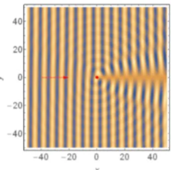
(4) 71. In Figure 1, we give the density plot of the real part of. $\varphi$-. in the case the momentum of the incident wave \mathrm{p} (1,0) and $\alpha$=1/2 . The arrow indicates the incident direction. We observe =. the difference between the phase of $\varphi$_{-} above and below the pos‐ itive x ‐axis. This reflects the singular behavior of the scattering. amplitude in the formula (3) at. $\theta$. = $\tau$. , caused by the magnetic. >_{\mathrm{s}. flux at the origin.. Figure 1: The density plot of {\rm Re} $\varphi$-\cdot. 3. Scattering by. N. solenoids in \mathbb{R}^{2}. Next, we consider the case there are is given by H_{N}=. N. solenoids (N\geq 2) perpendicular to the plane. The Hamiltonian. (\displaystyle \frac{1}{i}\nabla-A_{N})^{2}. on \mathb {R}^{2},. A_{N}=\displaystyle \sum_{j=1}^{N}A_{$\alpha$_{j} (x- _{j}. , y — yj) ,. (5). where A_{$\alpha$_{\mathrm{j} is the vector potential given in (1) with $\alpha$ $\alpha$_{j} , and 2 $\pi \alpha$_{j} is the magnetic flux through the solenoid at \mathrm{x}_{j} (x_{j}, y_{j}) (j = 1, \ldots, N) . We impose the regular boundary condition at each \mathrm{x}_{j}. Below we review the results of Ito‐Tamura [It‐Tal] and the author [Mi2], concerning the incoming wave =. =. solution and the scattering amplitude for the operator H_{N}.. 3.1. The result by Ito‐Tamura. In Ito‐Tamura [It‐Tal], they consider the case N=2, \mathrm{x}_{1} =O, \mathrm{x}_{2} =\mathrm{d} (\mathrm{d}\in \mathbb{R}^{2}\backslash \{O\}) , and calculate the asymptotics of the scattering amplitude as |\mathrm{d}|\rightarrow\infty . In this result, we identify an angle $\theta$\in[0, 2 $\pi$ ) 1 with a unit vector $\omega$ (coe $\theta$, \sin $\theta$ ) \in S^{1} (S_{1} \{ $\omega$ \in \mathbb{R}^{2} | $\omega$| and we denote f( $\omega$ \rightarrow$\omega$';k^{2}) instead of f( $\theta$\rightarrow$\theta$';k^{2}) . For \mathrm{x}\in \mathbb{R}^{2}\backslash \{0\} and $\omega$\in S^{1} , let $\gamma$(\mathrm{x}; $\omega$) denotes the azimuth angle of \mathrm{x} from the direction $\omega$ with 0\leq $\gamma$(\mathrm{x}; $\omega$)<2 $\pi$ . We use the notation =. =. =. \exp(i$\alpha\gam a$(\mathrm{x};$\omega$)=\left\{ begin{ar y}{l \exp(i$\alpha\gam a$(\mathrm{x};$\omega$) &(\mathrm{x}/|\mathrm{x}|\neq$\omega$),\ (1+\exp(2$\pi$ \alpha$)/2&(\mathrm{x}/|\mathrm{x}|=$\omega$), \end{ar y}\right.. \exp(i $\alpha \tau$(\mathrm{x}; $\omega$, $\omega$ =\exp(i $\alpha \gamma$(\mathrm{x}; $\omega$))\exp(i $\alpha \gamma$(\mathrm{x};-$\omega$')). .. Theorem 3.1 (Ito‐Tamura [It‐Tal]). Let f_{j}( $\omega$\rightarrow$\omega$';k^{2}) be the scattering amplitude by the single solenoid at \mathrm{x}_{j} with flux 2 $\pi$ a_{j} (j = 1,2) (f_{2} depends on d), and f_{\mathrm{d} ( $\omega$ \rightar ow $\omega$';k^{2}) be the scattering amplitude by the two solenoids. Then, for $\omega$\neq$\omega$', f_{\mathrm{d} ( $\omega$\rightar ow$\omega$';k^{2}) behaves like. f_{\mathrm{d} ( $\omega$\rightarrow$\omega$';k^{2}) = \exp(ia_{2} $\tau$(-\mathrm{d}; $\omega,\omega$'))f_{1}( $\omega$\rightarrow$\omega$';k^{2}) + \exp(i$\alpha$_{1} $\tau$(\mathrm{d}; $\omega,\omega$'))f_{2}( $\omega$\rightarrow$\omega$';k^{2})+o(1) as |\mathrm{d}|\rightar ow\infty with fixed. (6). \hat{\mathrm{d} =\mathrm{d}/|\mathrm{d}|.. The phase factors in the right hand side of (6) are considered to be an appearance of the AB‐effect. Actually, Kostrykin‐Schrader [Ko‐Sc] also study a large distance limit of the scattering amplitude for the Schrödinger operator H_{\mathrm{d}}=- $\Delta$+V_{1}+V_{2}(\cdot-\mathrm{d}) , and there is no such phase factor like (6) in their formula [\mathrm{K}+\mathrm{S}\mathrm{c}, (1.19)] . In Ito‐Tamura [It‐Ta2], they also consider the case N\geq 3..

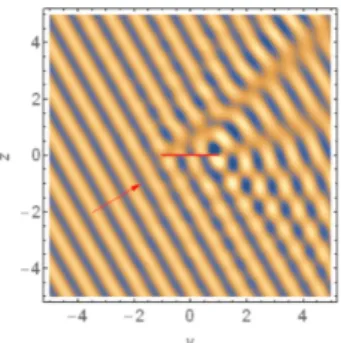
(5) 72. 3.2. Formulas in the elliptic coordinate. N 2, \mathrm{x}_{1} (-a, 0) and \mathrm{x}_{2} (a, 0) for some a > 0 , we can analyze the operator H_{2} by using the elliptic coordinate. This idea is used in Gu‐Qian [Gu‐Qi], and further developed by the author [Mil, Mi2]. For the detail in this subsection, see [Mil, Mi2]. For the Mathieu functions, see Abramowitz‐Stegun [Ab‐St] or McLachlan [Mc].. In the case. =. =. =. The elliptic coordinate is defined by. \left\{ begin{ar y}{l x=a\cosh$\xi$\cos$\eta$,\ y=a\sinh$\xi$\sin$\eta$, \end{ar y}\right.. $\xi$\geq 0, - $\pi$< $\eta$\leq $\pi$,. where a is a positive constant. The coordinate curves $\xi$= const. are confocal ellipses, and $\eta$= const. confocal hyperbolas. In the $\lambda$ u (An be elliptic coordinate, the Helmholtz equation −Au solved by separation of variables. The solutions are =. u=\mathrm{C}\mathrm{e}_{n}( $\xi$, q)\mathrm{c}\mathrm{e}_{n}( $\eta$, q) (n=0,1,2 u=\mathrm{S}\mathrm{e}_{n}( $\xi$, q)\mathrm{s}\mathrm{e}_{n}( $\eta$, q) (n=1,2, . .. ,. .. .. Figure 2: Elliptic coordinate.. where q=a^{2} $\lambda$/4 . The functions \mathrm{c}\mathrm{e}_{n} and \mathrm{s}\mathrm{e}_{n} are called the Mathieu functions, and \mathrm{C}\mathrm{e}_{n} and \mathrm{S}\mathrm{e}_{n} are called the modified Mathieu functions. The angular functions \mathrm{c}\mathrm{e}_{n} and \mathrm{s}\mathrm{e}_{n} are similar to the trigonometric functions, e.g., \mathrm{c}\mathrm{e}_{n} and \mathrm{C}\mathrm{e}_{n} are even functions, and \mathrm{s}\mathrm{e}_{n} and \mathrm{S}\mathrm{e}_{n} are odd functions. When N=2, \mathrm{x}_{1}=(-a, 0) and \mathrm{x}_{2}=(a, 0) , the AB Hamiltonian H_{2} is represented as. H_{2}=e^{i($\alpha$_{1}$\theta$_{1}+$\alpha$_{2}$\theta$_{2})}(- $\Delta$)e^{-i($\alpha$_{1}$\theta$_{1}+$\alpha$_{2}$\theta$_{2})}, $\theta$_{1}=\arg((x+a)+yi) , $\theta$_{2}=\arg((x-a)+yi). .. Put v=e^{-i($\alpha$_{1}$\theta$_{1}+$\alpha$_{2}$\theta$_{2})}\mathrm{u} . Then, the eigenequation H_{2}u= $\lambda$ u is equivalent to - $\Delta$ v= $\lambda$ v , but v becomes a multi‐valued function unless a_{1} and a_{2} are integers. Analyzing the latter equation, we conclude the eigenequation H_{2}u= $\lambda$ u can be solved by separation of variables in the elliptic coordinate if and only if. $\alpha$_{1}, $\alpha$_{2}\in(1/2)\mathbb{Z} .. (7). $\pi$ The condition (7) is called the magnetic quantization condition, since 2 $\pi$ (1/2) is equal to the quantum of magnetic flux h/(2e) under our normalization \hslash=h/(2 $\pi$)=1 and e=1 . In the case both $\alpha$_{1} and $\alpha$_{2} are odd multiples of 1/2, the solutions are =. u=e^{i($\alpha$_{1}$\theta$_{1}+$\alpha$_{2}$\theta$_{2})} $\Gamma$ \mathrm{e}_{n}( $\xi$, q)\mathrm{c}\mathrm{e}_{n}( $\eta$, q) (n=0,1,2_{\rangle} u=e^{i($\alpha$_{1}$\theta$_{1}+$\alpha$_{2}$\theta$_{2})}\mathrm{G}\mathrm{e}_{n}( $\xi$, q)\mathrm{s}\mathrm{e}_{n}( $\eta$, q) (n=1,2 ,. .. .. .. .. where q=a^{2} $\lambda$/4 . The functions \mathrm{F}\mathrm{e}_{n} and \mathrm{C}\mathrm{e}_{n} satisfy the same ordinary differential equation with respect to $\xi$ , but \mathrm{F}\mathrm{e}_{n} has the opposite parity to that of \mathrm{C}\mathrm{e}_{n} , that is, \mathrm{C}\mathrm{e}_{n} is even and \mathrm{F}\mathrm{e}_{n} is odd. The same relation holds for \mathrm{G}\mathrm{e}_{n} and \mathrm{S}\mathrm{e}_{n}.. We introduce the normalized modified Mathieu functions \mathrm{J}\mathrm{c}_{n}, \mathrm{J}\mathrm{s}_{n}, \mathrm{J}\mathrm{f}_{n} , and \mathrm{J}\mathrm{g}_{n} , which are constant multiples of \mathrm{C}\mathrm{e}_{n}, \mathrm{S}\mathrm{e}_{n}, \mathrm{F}\mathrm{e}_{n} , and \mathrm{G}\mathrm{e}_{n} , respectively, and behave like. \displaystyle \mathrm{J}\mathrm{c}_{n}( $\xi$, q)\sim \mathrm{J}\mathrm{s}_{n}( $\xi$, q)\sim\sqrt{\frac{2}{ $\pi$ kr} \cos(kr-\frac{n $\pi$}{2}-\frac{ $\pi$}{4}) \displaystyle \mathrm{J}\mathrm{f}_{n}( $\xi$, q)\sim\sqrt{\frac{2}{ $\pi$ kr} \cos(kr-\frac{n $\pi$}{2}-\frac{ $\pi$}{4}+$\delta$_{n,k}) \displaystyle \mathrm{J}\mathrm{g}_{n}( $\xi$, q)\sim\sqrt{\frac{2}{ $\pi$ kr} \cos(kr-\frac{n $\pi$}{2}-\frac{ $\pi$}{4}+$\epsilon$_{n,k}) as $\xi$\rightar ow. \infty. , where. q=a^{2}k^{2}/4 and. r=a. ,. \cosh $\xi$\sim |\mathrm{x}| . The first formula means \mathrm{J}\mathrm{c}_{n} and \mathrm{J}\mathrm{s}_{n} have the. same asymptotics as that of the Bessel function \mathrm{J}_{n} . The constants $\delta$_{n,k} and shifts in this context, which can be computed at least numerically.. $\epsilon$_{n,k}. are the scattering phase.

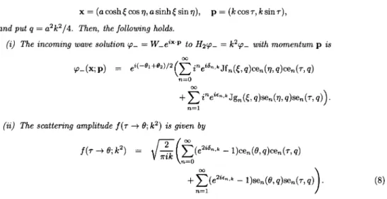
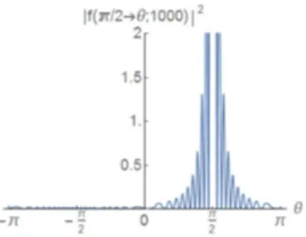
(6) 73. Theorem 3.2 ([Mi2]). Assume N=2,. use the elliptic coordinate in \mathrm{x}=. and put. \mathrm{x}. \mathrm{x}_{1}. =(-a, 0) , \mathrm{x}_{2}=(a, 0) ,. ‐space and the polar coordinate in. ( a \cosh $\xi$\cos $\eta$ , asinh $\xi$\sin $\eta$ ),. \mathrm{p}=. $\alpha$_{1}. \mathrm{p} ‐space,. =-1/2 , and. $\alpha$_{2}. that is,. =1/2 . We. ( k\cos $\tau$ , ksin $\tau$ ),. q=a^{2}k^{2}/4 . Then, the following holds.. (i) The incoming wave solution $\varphi$_{-}=W_{-}e^{i\mathrm{x}\cdot \mathrm{p} to H_{2}$\varphi$_{-}=k^{2}$\varphi$_{-} with momentum. is. \mathrm{p}. $\varphi$_{-}(\displaystyle\mathrm{x};\mathrm{p})=e^{i(-$\theta$_{1}+$\theta$_{2})/2}(\sum_{n=0}^{\infty}i^{n}e^{i$\delta$_{rk},\mathrm{J}\mathrm{f}_{n}($\xi$,q)\mathrm{c}\mathrm{e}_{n}($\eta$,q)\mathrm{c}\mathrm{e}_{n}($\tau$,q) +\displayst le\sum_{n=1}^{\infty}i^{n}e^{i$\epsilon$_{$\iota$,k}\prime}\mathrm{J}\mathrm{g}_{n}($\xi$,q)\mathrm{s}\mathrm{e}_{n}($\eta$,q)\mathrm{s}\mathrm{e}_{n}($\tau$,q). .. (ii) The scattering amplitude f( $\tau$\rightarrow $\theta$;k^{2}) is given by. f($\tau$\displaystyle\rightar ow$\theta$;k^{2})=\sqrt{\frac{2}{$\pi$ik}(\sum_{n=0}^{\infty}(e^{2i$\delta$_{n,k}-1)\mathrm{c}\mathrm{e}_{n}($\theta$,q)\mathrm{c}\mathrm{e}_{n}($\tau$,q) +\displayst le\sum_{n=1}^{\infty}(e^{2i$\epsilon$_{$\iota$,k}\prime}-1)\mathrm{s}\mathrm{e}_{n}($\theta$,q)\mathrm{s}\mathrm{e}_{n}($\tau$,q). .. (8). Formally the formula (8) is obtained by replacing \infty \mathrm{s}n $\theta$ by \mathrm{c}\mathrm{e}_{n}( $\theta$, q) , \sin n $\theta$ by \mathrm{s}\mathrm{e}_{n}( $\theta$, q) , and $\delta$_{m,k} by $\delta$_{n,k} or $\epsilon$_{n,k} , in the formula (4) (the term m=0 needs a slight modification). Actually, both formulae can be proved by the plane wave expansion formula rin each coordinate. In Figure 3‐4, we give the density plots of the real part of the incoming wave solutions for k=4 and $\tau$=0, $\pi$/2 , which describe the AB‐phase shift in this model. In Figure 5 and 6, we give the graphs of the differential scattering cross sections (DSCS) |f( $\tau$\rightarrow $\theta$;1000)|^{2} obtained by the Ito‐Tamura asymptotic formula (6) and that by the elliptic coordinate (8), respectively. A small difference is seen near $\theta$=0 , which is the direction of \mathrm{d}=\mathrm{x}_{2}-\mathrm{x}_{1} , where the convergence of the Ito‐Tamura formula (6) is not uniform.. \sim. \sim. -4. -2. 0. 2. 4. -4. -2. 0. \mathrm{x}. Figure 3: Plot of {\rm Re}$\varphi$_{-} , for k=4,. 4 4.1. 2. 4. x. $\tau$=0.. Figure 4: Plot of {\rm Re}$\varphi$_{-} , for k=4, $\tau$= $\pi$/2.. Scattering by the toroidal magnetic field in \mathb {R}^{3} The result by Ballesteros‐Weder. In Ballesteros‐Weder [Ba‐We2], they study the Schröùnger operator with the magnetic field enclosed inside the torus. T=\{(x, y, z)\in \mathbb{R}^{3}|R_{1}^{2}\leq|x|^{2}+|y|^{2}\leq R_{2}^{2}, |z|\leq H\}.

(7) 74. 1. z. 1. 1. Figure 5: DSCS by the Ito‐Tamura formula,. Figure 6: DSCS by the elliptic coordinate,. $\tau$= $\pi$/2.. $\pi$/2.. $\tau$=. for some 0<R_{1} <R_{2} and H>0 . Put. $\Omega$=\mathbb{R}^{3}\backslash (T\cup S) , S=\{(x, y, z)\in \mathbb{R}^{3}| |x|^{2}+|y|^{2}>R_{2}^{2}, z=0\}. Since. $\Omega$. is simply connected, in the set. $\Omega$. the magnetic Schrödinger operator. H= $\Phi$ H_{0}$\Phi$^{-1}, H_{0}=- $\Delta$ , by some gauge function $\varphi$_{\mathrm{v}. $\Phi$. going through the hole of the torus with velocity. H. is represented as. (see (10) below). So, for a Gaussian wave packet \mathrm{v}. , we can use the approximation. e^{-itH}$\varphi$_{\mathrm{v} $\Phi$ e^{-itH_{0} $\Phi$^{-1}$\varphi$_{\mathrm{v} . This kind of approximation is also used by Aharonov‐Bohm [\mathrm{A}\mathrm{h}-\mathrm{B}\mathrm{o}]_{\rangle} so Ballesteros‐Weder call the approximation Aharonov‐Bohm ansatz. Ballesteros‐Weder give a very precise error estimate for this. approximation under the situation of the experiment by Tonomura et al. [Ba‐We2, Theorem 1.1], which. justifies the experiment qualitatively.. 4.2. Infimitesimally thin ring magnetic field. Here we take another approach to this problem. consider a ring R of thickness 0 in \mathbb{R}^{3} , given by. We. R=\{\mathrm{x}=(x, y,0)\in \mathbb{R}^{3}||\mathrm{x}|=a\}, for some. a>0 .. We consider the magnetic Schrödinger. operator H=. (\displaystyle \frac{1}{i}\nabla -A)^{2}. R. Figure 7: Zero thickness ring magnetic field. on. \mathb {R}^{3},. where A\in C^{\infty}(\mathbb{R}^{3}\backslash R;\mathbb{R}^{3}) is the magnetic vector po‐ tential satisfying \nabla\times A=0. in. \mathbb{R}^{3}\backslash R,. \displaystyle \int_{D}(\nabla\times A)\cdot \mathrm{n}dS=\int_{\partial D}A\cdot d\el =0$\pi$_{\rangle}. (9). for any small disc D pierced by the ring R , where 0 is an odd integer, and \mathrm{n} is the unit normal vector on D. (the direction of \mathrm{n} is appropriately fixed), with supp A bounded set in \mathbb{R}^{3} (9) is the magnetic quantization condition in this context.. Figure 8: The oblate spheroidal coordinate.. We impose the regular boundary condition along R , or more precisely, H is the Friedrichs extension of the operator H|_{C_{0}^{\infty}(\mathrm{R}^{3}\backslash R)} . This is an idealized model to the experiment by Tonomura et al., and the.

(8) 75. advantage is that this model is explicitly solvable in the oblate spheroidal coordinate, defined as follows.. where. \left{begin{ar y}l x=a\cosh$\xi sn$\eta cos$\phi,\ y=a\cosh$\xi sn$\eta sin$\phi,\ z=a\sinh$\xi cos$\eta, \end{ar y}\ight. \left(bgin{ary}{l $\xi&\geq0\ 0\leq&$\eta leq$\pi -$\pi<$\phi leq$\pi& \end{ary}\right). a. is a positive constant. The surface $\xi$=const . is a flattened elhpsoid, $\eta$=const . a hyperboloid. of one sheet, $\phi$=const . a half‐plane (see Figure 8). In the oblate spheroidal coordinate, the equation - $\Delta$ u=k^{2}u can be solved by separation of variables, and the solutions are. \cos $\eta$)R_{m\ell}^{(1)} (‐iak, isinh $\xi$ ) \cos m$\phi$_{j} u=S_{m\ell}( ‐iak, \cos $\eta$)R_{m\ell}^{(1)} (‐iak, isinh $\xi$ ) \sin m $\phi$ u=S_{m\ell} ( ‐iak,. (m=0,1,2,. \ell=m, m+1, m+2,. \ldots,. where S_{m\ell} is the angular spheroidal wave function, and. R_{m\ell}^{(1)}. .. (m\neq 0) ,. .. the radial spheroidal wave function of the. first kind. For the detail of these functions, see Abramowitz‐Stegun [Ab‐St] or Flammer [F1]. Take. \mathrm{x}_{0}. \in \mathbb{R}^{3} sufficiently large, and put. $\Phi$(\displaystyle \mathrm{x})=\exp(i\ nt_{\mathrm{x}_{0} ^{\mathrm{x} A\cdot d\el ) (\mathrm{x}\in \mathb {R}^{3}) where the path of the integral is in the region \mathbb{R}^{3}\backslash R . The function. ,. $\Phi$. is two‐valued, since. \displaystyle \exp(i\int_{\partial D}A\cdot d\el ) =e^{io $\pi$}=-1 for any small disc. D. pierced by the ring. R.. Moreover, we have. Hu= $\Phi$(-\triangle)$\Phi$^{-1}u .. (10). Then, as in the two‐dimensional case, the solutions to Hu=k^{2}u are given as. \cos $\eta$)R_{m\ell}^{(5)} (‐iak, isinh $\xi$ ) \cos m $\phi$, u= $\Phi$\cdot S_{m\ell} ( ‐iak, \cos $\eta$)R_{m\ell}^{(5)} (‐iak, isinh $\xi$ ) \sin m $\phi$ u= $\Phi$\cdot S_{m\ell} ( ‐iak,. (m\neq 0) ,. (m=0,1,2, \ldots, \ell=m, m+1, m+2, \ldots.). The functions R_{m\ell}^{(1)}(c, z) and R_{m\ell}^{(5)}(c, z) ( c= −iak) satisfy the same ordinary differential equation with re‐ spect to z , and have different parities. Both functions $\Phi$ and S_{m\ell} ( ‐iak, \cos $\eta$)R_{m\ell}^{(5)} (‐iak, isinh $\xi$ ) \cos m $\phi$ \sin m $\phi$ ) are two‐valued with respect to the original coordinate x , and the product of these func‐ (or tions is single‐valued. The scattering phase shift. $\delta$_{\el ,k}^{m} is defined by the asymptotics. R_{m\el }^{(1)}(c, z)\displaystyle \sim\frac{1}{cz}\cos(cz-\frac{\el +1}{2} $\pi$) R_{m\el }^{(5)}(c, z)\displaystyle \sim\frac{1}{CZ}\cos(cz-\frac{\el +1}{2} $\pi$+$\delta$_{l,k}^{m}) ,. as. z. \rightarrow. i\infty .. When. c. =. −iak and. z. =. isinh $\xi$ , we have. cz=. k. a \sinh $\xi$ \sim kr (r = |\mathrm{x}|) and the. limit corresponds the limit . Thus R_{m\ell}^{(1)}(c, z) has the same asymptotic behavior as the asymptotics of the spherical Bessel function. Our main result is formulated as follows. z\rightarrow i\infty. Theorem 4.1. coordinate in. r\rightarrow\infty. (i) We introduce the oblate spheroidal coordinate in \mathrm{p} ‐space,. \mathrm{x}. ‐space and the spherical. that is, \mathrm{x}=. \mathrm{p}=. ( a \cosh $\xi$\sin $\eta$\cos $\phi$ , acosh $\xi$\sin $\eta$\sin $\phi$ , asinh $\xi$\cos $\eta$ ), ( k\sin $\tau$\cos $\psi$ , ksin $\tau$\sin $\psi$ , kcos $\tau$ )..

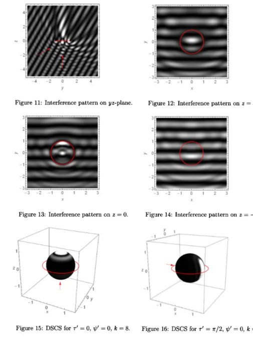
(9) 76. Then, the incoming wave solution netic fidd \dot{u}. $\varphi$_{-}(\mathrm{x};\mathrm{p}). =. $\varphi$_{-}. =W_{-}e^{i\mathrm{x}\cdot \mathrm{p} with momentum. $\Phi$\displayst le\cdot\sum_{m=0}^{\infty}\sum_{\el=m}^{\infty}i^{\el}c_{l,m}^{2}e^{i$\delta$_{p}^{rn_{k} ,R_{m\el}^{(5)}. \mathrm{p}. for the quantized ring mag‐. (‐iak, isinh $\xi$ ). S_{m\ell} ( ‐iak, \cos $\eta$)S_{ $\pi$ d}( ‐iak, \cos $\tau$)\cos(m( $\phi$- $\psi$)) ,. c_{\ell,m}=\sqrt{(2-$\delta$_{0m})(2\ell+1)(\ell-m)!}/(P+m)!.. where. (ii) We introduce the spherical coordinate in S^{2} as $\omega$=(\sin $\tau$\cos $\psi$, \sin $\tau$\sin $\psi$, \cos $\tau$). ,. $\omega$'=(\sin$\tau$'\cos$\psi$', \sin$\tau$'\sin$\psi$', \cos$\tau$') for. $\omega$,. $\omega$' \in S^{2}. magnetic field is. Then, the scattering amplitude with energy k^{2} (k > 0) for the quantized ring. f($\omega$'\displaystyle\rightar ow$\omega$;k^{2})=\frac{1}{2ik}\sum_{m=0}^{\infty}\sum_{\el=m}^{\infty}(e^{2i$\delta$_{\el,\mathrm{k}^{lr$\iota$}-1)c_{\el,m}^{2}. S_{ml} ( ‐iak, \cos $\tau$)S_{m\ell}( ‐iak, \cos$\tau$')\cos(m( $\psi$- $\psi$. where. c_{\ell,m}. is as in (i).. Let us try to reproduce the interference pattern in the experiment by Tonomura et al. by using 1 , and consider the object wave $\varphi$-,1 W_{-}e^{i\mathrm{p}_{1}\cdot \mathrm{x} with the incident the above formula. We put a momentum \mathrm{p}_{1}=(0,0,8) , which goes through the hole of the ring solenoid vertically. We also consider =. the reference wave. $\varphi$_{-,2}=W_{-}e^{i\mathrm{p}_{2}\cdot \mathrm{x}. =. with \mathrm{p}_{2}. =(0,4\sqrt{3},4) .. The two vectors \mathrm{p}_{1} and \mathrm{p}_{2} have the same. length, and make the angle $\pi$/3 . The density plot of the real part of $\varphi$_{-,1} and that of $\varphi$_{-,2} on the yz‐plane are given in Figure 9, 10, respectively. The central segment represents the ring R . We observe the phase shift occurs behind the ring, depending on the incident direction of the electron beam. In these figures, we take $\Phi$=1 for simplicity, so $\varphi$-,j are discontinuous on the disc enclosed by the ring.. \mathrm{N}. \mathrm{M}. -4. -2. 0. 2. 4. y. Figure 9: The density plot of {\rm Re}$\varphi$_{-,1}.. Figure 10: The density plot of {\rm Re}$\varphi$_{-,2}.. Of course, the real part of the wave function is gauge‐dependent, and not an observable quantity. The interference pattern caused by the superposition of these two waves is defined by |$\varphi$_{-,1}+$\varphi$_{-,2}|^{2}, which is a gauge‐independent quantity. In Figure 11‐14, we give the density plots of the interference pattern on several planes. Especially, Figure 12, the interference pattern behind the ring magnet, is similar to the picture by Tonomura et al. We also give the spherical density plots of the differential scattering cross section |f( $\omega$'\rightarrow $\omega$;k^{2})|^{2} in Figure 15 and 16..

(10) 77. At present we do not have an asymptotic formula for the scattering amplitude in the high energy limit in terms of elementary functions, like the Ito‐Tairiura formula (6). To our knowledge, the only known result is the Aharonov‐Bohm ansatz by Ballesteros‐Weder [Ba‐We2]; when the velocity \mathrm{v} is directed. to the z ‐axis, the scattering operator acts on the Gaussian wave packet. $\varphi$_{\mathrm{v}. as the multiplication by. \exp(2 $\pi \alpha$ i) ( 2 $\pi \alpha$ is the magnetic flux through the section of the torus) in the high energy limit. Finding more general asymptotic formula, which explains Figure 9 and 10 more clearly, is an interesting problem. In the computational side, the rapid computation of the spheroidal wave function is desired recently,. mainly in application to the signal processing analysis (see e.g. Kirby [Kil, Ki2. We hope the progress. in this area, which will give us more detailed information about our scattering problem.. \mathrm{N}. \sim. -4. -2. 0. 2. 4. -3 -2 -1 0 1 2 3. $\gamma$. \mathrm{x}. Figure 11: Interference pattern on yz‐plane.. \sim. Figure 12: Interference pattern on. z=3.. \Rightarrow. -3. -2. -1. 0. I. 2. 3. -3 -2 -1 0 1 2 3. $\chi$. $\chi$. Figure 13: Interference pattern on. z=0.. Figure 15: DSCS for $\tau$'=0, $\psi$'=0,. k=8.. Figure 14: Interference pattern on. z=-2.. Figure 16: DSCS for $\tau$'= $\pi$/2, $\psi$'=0,. k=8..

(11) 78. References [Ab‐St]. M. Abramowitz and I. A. Stegun, Handbook of mathematical fúnctions with formulas, graphs, and mathematical tables, National Bureau of Standards Applied Mathematics Series, 55 U.S. Government Printing Office, Washington, D.C. 1964.. [Ah‐Bo] Y. Aharonov and D. Bohm, Significance of electromagnetic potentials in the quantum theory, Phys. Rev. 115 (1959) 485‐491.. [Ar]. S. Arians, Geometric approach to inverse scattering for the Schrödinger equation with magnetic and electric potentials, J. Math. Phys. 38 (1997), no. 6, 2761‐2773.. [Ba‐Wel] M. Ballesteros and R. Weder, High‐velocity estimates for the scattering operator and Aharonov‐Bohm effect in three dimensions Comm. Math. Phys. 285 (2009), no. 1, 345‐398.. [Ba‐We2] M. Ballesteros and R. Weder, The Aharonov‐Bohm effect and Tonomura et al. experiments: rigorous results. J. Math. Phys. 50 (2009), no. 12, 122108, 54 pp. [Ba‐We3] M. Ballesteros and R. Weder, Aharonov‐Bohm effect and high‐velocity estimates of solutions to the Schrödinger equation, Comm. Math. Phys. 303 (2011), no. 1, 175‐211. [Esl]. G. Eskin, Inverse boundary value problems and the Aharonov‐Bohm effect, Inverse Problems 19 (2003), no. 1, 49‐62.. [Es2]. G. Eskin, Inverse problems for the Schrödinger equations with time‐dependent electromagnetic potentials and the Aharonov‐Bohm effect, J. Math. Phy\mathcal{S}. 49 (2008), no. 2, 022105, 18 pp.. [Es3]. G. Eskin, Aharonov‐Bohm effect revisited, Rev. Math. Phys. 27 (2015), no. 2, 1530001, 52 pp.. [Es‐Is‐Od] G. Eskin, H. Isozaki, and S. O’Dell, Gauge equivalence and inverse scattering for Aharonov‐ Bohm effect, Comm. Partial Differential Equations 35 (2010), no. 12, 2164‐2194.. [F1]. C. Flammer, Spheroidal Wave Functions, Stanford Univ. Press, 1957.. [Gu‐Qi] Zhi‐Yu Gu and Shang‐Wu Qian, Aharonov‐Bohm scattering on parallel flux hnes of the same magnitude, J. Phys. A: Math. Gen. 21 (1988), 2573‐2585. [He]. B. Helffer, Introduction to some conjectures for spectral minimal partitions, J. Egyptian Math. Soc. 19 (2011), 45‐51.. [It‐Tal] H. T. Ito and H. Tamura, Aharonov‐Bohm effect in scattering by point‐like magnetic fields at large separation, Ann. Henri Poincare 2 (2001), no. 2, 309‐359. [It‐Ta2] H. T. Ito and H. Tamura, Aharonov‐Bohm effect in scattering by a chain of point‐like magnetic fields, Asymptot. Anal. 34 (2003), no. 3‐4, 199‐240.. [Iw‐Mi‐Sh] A. Iwatsuka, T. Mine, and S. Shimada, Norm resolvent convergence to Schrödinger oper‐ ators with infinitesimally thin toroidal magnetic fields, in Spectral and Scattering Theory for. Quantum Magnetic Systems, Contemporary Mathematics 500 (2009), AMS, 139‐152.. [Kil]. P. Kirby, Calculation of spheroidal wave functions, Comput. Phys. Comm. 175 (2006), 465‐472.. [Ki2]. P. Kirby, Calculation of radial prolate spheroidal wave functions of the second kind, Comput. Phys. Comm. 181 (2010), 514‐519. \check{}. [Ko‐Stl] P. Kocábová and P. Št ovíček, Generalized Bloch analysis and propagators on Riemanman manifolds with a discrete symmetry, J. Math. Phys. 49 (2008), no. 3, 033518, 16 pp. \check{}. [Ko‐St2] P. Košt áková and P. Štoviček, Noncommutative Bloch analysis of Bochner Laplacians with nonvanishing gauge fields, J. Geom. Phys. 61 (2011) , no. 3, 727‐744..

(12) 79. [Ko‐Sc] V. Kostrykin and R. Schrader, Cluster properties of one particle Schrödinger operators. II, textitRev. Math. Phys. 10 (1998), no. 5, 627‐683. [Mc]. N. W. McLachlan, Theory and Application of Mathieu Functions, Oxford, at the Clarenden Press, 1947.. [Mil]. T. Mine, Solvable models in two‐solenoidal Aharonov‐Bohm magnetic fields on the Euclidean plane, RIMS Kôkyûroku Bessatsu B45, 45‐68.. [Mi2]. T. Mine, Solvable models in the spheroidal coordinates (Japanese), Mathematical Aspects of Quantum Fields and Related Topics, RIMS Kôkyûroku 1961 (2014), 56‐73.. [Ru]. S. N. M. Ruijsenaars, The Aharonov‐Bohm Effect and Scattering Theory, Ann. Phys. 146. (1983), 1‐34.. [Na]. Y. Nambu, The Aharonov‐Bohm problem revisited, Nuclear Phys. B 579 (2000), no. 3, 590‐ 616.. [Ni]. $\Gamma$ .. [Pe‐To]. M. Peshkin and A. Tonomura, The Aharonov‐Bohm effect, Lec. Notes Phys. 340, Springer,. Nicoleau, An inverse scattering problem with the Aharonov‐Bohm effect, J. Math. Phys. 41. (2000), no. 8, 5223‐5237. 1989. \check{}. [St]. P. Št ovíček, The Green function for the two‐solenoid Aharonov‐Bohm effect, Phys. Lett. A 142. [To]. A. Tonomura et al., Evidence for Aharonov‐Bohm Effect with Magnetic Field Completely. (1989), no. 1, 5‐10.. Shielded from Electron Wave, Phys. Rev. Lett. 56, No. 8 (1986), 792‐795. [Ro‐Ya] Ph. Roux and D. Yafaev, On the mathematical theory of the Aharonov‐Bohm effect, J. Phys. A 35 (2002), no. 34, 7481‐7492. [We]. R. Weder, The Aharonov‐Bohm effect and time‐dependent inverse scattering theory, Inverse Problems 18 (2002), no. 4, 1041‐1056.. [Ya]. D. R. Yafaev, Scattering by magnetic fields (Russian), Algebra i Analiz 17 (2005), no. 5, 244−272; translation in St. Petersburg Math. J. 17 (2006), no. 5, 875‐895..

(13)