Partitioned Runge-Kutta methods for partial differential equations (The Numerical Solution of Differential Equations and Linear Computation)

(1)

Partitioned Runge-Kutta methods for

partial

differential equations

TOSHIYUKI Koto 小藤俊幸

Department of Computer Science

The University of ElectrO-Communications

電気通信大学情報工学科

e-mail:[email protected]

Abstract

We consider implicit-explicit Runge-Kutta (IMEX$\mathrm{R}\mathrm{K}$) schemes for

time-dependent semi-linear partial differential equations. We show that theerrorof

ascheme isof$O(\Delta t^{2})$ in time undersomeconditions, whereAt isthestepsize.

This result is, in asence, optimal. The s0-called order reduction phenomena

occur, i.e., the error of ascheme based on apartitioned RK method whose

order $\geq 3$ behaves as $O(\Delta t^{2})$, which is shown numerically.

1. Introduction

We consider initial-boundary value problems of the form

$\frac{\partial u}{\partial t}=Lu+g(t, x, u)$, $0\leq t\leq T$, $x\in\Omega$, (1.1)

$\Phi_{b}u(t, x)=\varphi(t, x)$, $0\leq t\leq T$, $x\in\partial\Omega$, (1.2)

$u(0, x)=u^{0}(x)$, $x\in\Omega$. (1.3)

Here, $u=u(t, x)$ is an $R^{m}$-valued unknown function, $\Omega$ is abounded domain in

$R^{d}$ with the boundary

an,

$L$ is alinear partial differential operator with constant

coefficients with respect to $x$, $\Phi_{b}$ is aboundary operator. Various reaction-diffusion

equations andnonlinearSchrodingerequations such

as

theGross-Pitaevskii equation

(see, e.g., [4]) are typical examples of (1.1).

Manynumerical schemes for evolutionalproblems inpartial differential equations

(PDEs)

are

derived and implemented along the idea of the method of lines (MOL).

In this approach aPDE is first discretized in space by finite difference or finite

element techniques to be converted into asystem of ordinary differential equations

(ODEs). We consider the grid $\Omega_{h}$ defined by $\Omega_{h}=\Omega\cap hZ^{d}$ for $h>0$, and MOL

approximations of (1.1)-(1.2) in the form

$\frac{\mathrm{d}U_{h}}{\mathrm{d}t}=L_{h}U_{h}+\varphi_{h}(t)+g_{h}(t, U_{h})$

.

(1.4)

Here, $U_{h}$ is

an

approximate function of $u$ on $\Omega_{h}$, $L_{h}$ is adifference approximation

of $L$, _{$g_{h}$} is the restriction of

$g$ onto $\Omega_{h}$, and $\varphi_{h}(t)$ is afunction determined from the

boundary condition (1.2)

数理解析研究所講究録 1320 巻 2003 年 60-70

(2)

The ODE (1.4) is usually astiff equation, not easily treated with the standard

explicit methods. In some cases (e.g.,$[11])$, theequation (1.4) is solved by ascheme

of the form

$U_{h}^{n+1}=U_{h}^{n}+\Delta t(L_{h}U_{h}^{n+1}+\varphi_{h}(t_{n+1}))+\Delta tg_{h}(t_{n}, U_{h}^{n})$, (1.5)

where At is the stepsize, given by $\Delta t=T/N$for

some

integer $N$ $\geq 1$, $t_{n}=n\Delta t$, and

$U_{h}^{n}$ is an approximate value of$U_{h}(t_{n})$

.

The scheme (1.5) is obtained by applying the

backward Euler formula to thelinear part of (1.4) and the forward Euler formulato

the nonlinear part. This type of scheme is called implicit-explicit (IMEX) scheme,

or semi-implicit scheme.

The scheme (1.5) is offirst order in the sense oforder ofconvergence. There are

two ways of improving (1.5) in accuracy:

one

is along the idea of linear multistep

methods [1, 3, 12]; the other is along the idea of Runge-Kutta (RK) methods [2, 6, 8].

We follow the latter approach.

Let us consider apair of two RK methods defined by the arrays

000.

.

0 000.

. .

0 $c_{2}$ $a_{21}$ $a_{22}$ 0

. . .

0 $c_{2}$ $\hat{a}_{21}$ 0

. . .

0 $c_{3}$ $a_{31}$ $a_{32}$ (Z33

.

$\cdot$

.

, $c_{3}$ $\hat{a}_{31}$ $\hat{a}_{32}$ 0 $.$

.

. (1.6) . $\cdot$

.

...

$\cdot.$

.

0

...

.

$\cdot$

.

...

0 $\mathrm{c}_{s}$ $a_{s1}$ $a_{s2}$

. . .

$a_{s,s-1}$ $a_{ss}$ $c_{s}$ $\hat{a}_{s1}$ $\hat{a}_{s2}$

. . .

$\hat{a}_{s,s-1}$ 0

$b_{1}$ $b_{2}$ $\cdots$ $b_{s-1}$ $b_{\mathit{8}}$ $\hat{b}_{1}$ $\hat{b}_{2}$

$\cdots$ $\hat{b}_{s-1}$ $\hat{b}_{s}$

0 $c_{2}$ $c_{3}$ $.\cdot$

.

$c_{s}$ 0 0 $\ldots$ 0 $a_{21}$ $a_{22}$ 0

. . .

0

$a_{31}$ $a_{32}$ $a_{33}$

.

$\cdot$

.

...

$\cdot$

..

0

$a_{s1}$ $a_{s2}$

...

$a_{s,s-1}$ $a_{ss}$

$b_{1}$ $b_{2}$

.

$b_{s-1}$ $b_{\mathit{8}}$ 0 $c_{2}$ $c_{3}$ $..$

.

$c_{s}$ 0 0 $\ldots$ 0 $\hat{a}_{21}$ 0

.

..

0 $\hat{a}_{31}$ $\hat{a}_{32}$ 0

...

.

$\cdot$

.

...

₀

$\hat{a}_{s1}$ $\hat{a}_{s2}$

. . .

$\hat{a}_{s,s-1}$ 0

$\hat{b}_{1}$ $\hat{b}_{2}$

.

..

$\hat{b}_{s-1}$ $\hat{b}_{s}$

The left formula determines adiagonally implicit (semi-implicit) RK method, the

right formula an explicit RK method. As usual, we

assume

that

$c_{i}= \sum_{j=1}^{i}a_{ij}=\sum_{=J1}^{i-1}\hat{a}_{ij}$, $0\leq c:\leq 1$, $i=2,3$, $\ldots$ , $s$. (1.7)

By applying the left formula to the linear part of (1.4) and the right formula to

the nonlinear part, we obtain the following scheme for the initial-boundary value

problem (1.1)-(1.2):

$U_{h,n}^{(*)}.=U_{h}^{n}+ \Delta t\sum_{j=1}^{i}a_{ij}(L_{h}U_{h,n}^{(j)}+\varphi_{h}(t_{n}+c_{j}\Delta t))$

$+ \Delta t\sum_{j=1}^{i-1}\hat{a}_{ij}g_{h}$

(

$t_{n}+c_{j}\Delta t$, $U_{h,n}^{(j)}$

),

$i=1,2$,

$\ldots$ , $s$, (1.8)

$U_{h}^{n+1}=U_{h}^{n}+ \Delta t\sum_{i=1}^{s}b_{i}(L_{h}U_{h,n}^{(i)}+\varphi_{h}(t_{n}+c_{i}\Delta t))$

$+\Delta t$$\sum_{i=1}^{s}\hat{b}_{i}g_{h}$

(

$t_{n}+c_{\dot{\iota}}\Delta t$,$U_{h,n}^{(\dot{|})}$

).

(1.9)

(3)

Here, $U_{h}^{0}$ is given by $U_{h}^{0}=[u^{0}(x)]_{x\in\Omega_{h}}$.

The main purpose of the present paper is to clarify the convergence property

of the scheme (1.8)-(1.9), especially from aviewpoint of the $B$-convergence theory

[7]. The concept of $B$-convergence is closely related to the s0-called order reduction

phenomena, which

were

first pointed out and studied by Verwer [15] in the PDE

context (see also [13, 14]).

2.

Main

theorem

For $\sigma^{m}$-valued functions

on

$\Omega_{h}$ we define

an

inner product by

$\langle U, V\rangle_{h}=h^{d}\sum_{x\in\Omega_{h}}\overline{U}(x)^{T}V(x)$, (2.1)

and let $||\cdot||_{h}$ denote the corresponding

norm.

We also put

$\alpha_{h}(t)=u_{h}’(t)-L_{h}u_{h}-\varphi_{h}(t)-g_{h}(t, u_{h})$, (2.2)

where $u_{h}(t)=[u(t, x)]_{x\in\Omega_{h}}$, and consider the following conditions concerning the

problem (1.1)-(1.3) and the MOL approximation (1.4)

$(\mathrm{A}_{1})$ The exact solution $u(t, x)$ is of class $C^{3}$ with respect to $t;g(t, x, u)$ is of class

$C^{2}$ with respect to $t$,_$u$ and the functions

g, $\frac{\partial g}{\partial t}$

, $\frac{\partial g}{\partial u_{i}}$ , $\frac{\partial^{2}g}{\partial t^{2}}$

, $\frac{\partial^{2}g}{\partial t\partial u_{i}}$ , $\frac{\partial^{2}g}{\partial u_{i}\partial u_{j}}$

are bounded for $(t, x, u)\in[0, T]\cross\Omega\cross R^{m}$.

$(\mathrm{A}_{2})$ For any $\sigma^{m}$-valued function $U$ on $\Omega_{h}$, ${\rm Re}\langle U, L_{h}U\rangle_{h}\leq 0$

.

(A3) $||\alpha_{h}(t)||_{h}arrow 0$ as $harrow 0$

.

Moreover we write

$A=(a_{ij})_{1\leq i,j\leq s}$, $b=[b_{1}, b_{2}, \ldots, b_{s}]^{T}$,

$\hat{A}=(\hat{a}_{\dot{|}j})_{1\leq i,j\leq s}$, $\hat{b}=[\hat{b}_{1}, \hat{b}_{2}, \ldots, \hat{b}_{s}]^{T}$,

and consider the following conditions concerning the RK pair (1.6).

$(\mathrm{B}_{1})$ The partitioned RK method (1.6) is of second order, i.e., the parameters $b_{i}$,

$\hat{b}_{i}$,

$c_{i}$.satisf

$\sum b_{i}=1$, $\sum_{i=1}^{s}b_{i}c_{i}=1/2$, $\sum_{i=1}^{s}\hat{b}_{i}=1$, $\sum_{i=1}^{s}\hat{b}_{i}c_{i}=1/2$

.

(4)

83

$(\mathrm{B}_{2})$ The diagonally implicit RK method is $A$-stable, $ASI$-stable, and AS-stable,

i.e., the stability function $r(z)=1+zb^{T}(I_{s}-zA)^{-1}1,1=[1,1, \ldots, 1]^{T}$,

satisfies

$|r(z)|\leq 1$ for any $z\in C_{-}$,

and each component of $(I_{s}-zA)^{-1}$ and $zb^{T}(I_{s}-zA)^{-1}$ is bounded on $\varpi_{-}$,

where $\Phi_{-}=\{z\in C : {\rm Re} z<0\}$.

(B3) The rational functions

$\phi(z)=\frac{b^{T}(I_{s}-zA)^{-1}\gamma}{b^{T}(I_{s}-zA)^{-1}1}$ , $\hat{\phi}(z)=\frac{b^{T}(I_{s}-zA)^{-1}\hat{\gamma}}{b^{T}(I_{s}-zA)^{-1}1}$ (2.3)

are bounded on $C_{-}$, where

$\gamma=[\gamma_{1}, \gamma_{2}, \ldots, \gamma_{s}]^{T}$, $\hat{\gamma}=[\hat{\gamma}_{1},\hat{\gamma}_{2}, \ldots,\hat{\gamma}_{s}]^{T}$,

$\gamma_{i}=c_{i}^{2}/2-\sum_{j=1}^{i}a_{ij^{C}j}$, $\hat{\gamma}_{i}=\mathrm{I}$$a_{ij}c_{j}- \sum_{j=1}^{i-1}\hat{a}_{j}\dot{.}c_{j}$.

Theorem 2.1 Assume that $(\mathrm{A}_{1})$ (B3) and $(\mathrm{B}_{1})$-(B3)are

satisfied.

Then, there are

positive numbers $h_{0}$, AtO, C such that

$1 \leq n\leq N\mathrm{m}\mathrm{a}\mathrm{x}||U_{h}^{n}-uh(tn)||_{h}\leq C(\triangle t^{2}+\max 0\leq t\leq_{-}T||\alpha_{h}(t)||_{h})$ (2.4)

holds

_for

any $h\leq h_{0}$ and $At\leq\Delta t\circ\cdot$

The proof is carried out by asimular argument as in the proof of Theorem 3.3

[5], on the based of the following lemma (see, e.g., [10], IV.II).

Lemma 2.2 (Theorem of

von

Neumann) Let$\psi(z)$ be a rational

function

which

has no pole in $C_{-}$, and assume that $L_{h}$

satisfies

$(\mathrm{A}_{2})$

.

Then, we have

$|| \psi(\Delta tL_{h})||_{h}\leq\sup_{{\rm Re} z\leq 0}|\psi(z)|$ . (2.5)

Proof of Theorem 2.1. Put $t_{n,i}=t_{n}+c_{i}\Delta t$ and define $r_{h,n}^{(i)}$,

$\rho_{h,n}$ by

$u_{h}(t_{n,i})=u_{h}(t_{n})+ \Delta t\sum_{j=1}^{i}a_{ij}(L_{h}u_{h}(t_{n,j})+\varphi_{h}(t_{n,j}))$

$+ \Delta t\sum_{j=1}^{i-1}\hat{a}_{\dot{\iota}j}g_{h}$

(

$t_{n,j}$, $u_{h}(t_{n,j}))+r_{h,n}^{(i)}$, (2.6)

$u_{h}(t_{n+1})=u_{h}(t_{n})+ \Delta t\sum_{i=1}^{s}b_{i}(L_{h}u_{h}(t_{n,i})+\varphi_{h}(t_{n,i}))$

$+ \Delta t\sum_{i=1}^{s}\hat{b}_{i}g_{h}$

(

$t_{n,i}$,$u_{h}(t_{n,i}))+\rho_{h,n}$. (2.7)

(5)

Then, it follows from (2.2) and (1.7) that

$r_{h,n}^{(i)}=u_{h}(t_{n,i})-u_{h}(t_{n})- \Delta t\sum_{\mathrm{j}=1}^{l}a_{ij}[u_{h}’(t_{n,j})-g_{h}(t_{n,j},$ $u_{h}(t_{n,j}))-\alpha_{h}(t_{n,j})]$

$- \Delta t\sum_{j=1}^{i-1}\hat{a}_{ij}g_{h}(t_{n,\mathrm{j}},$$u_{h}(t_{n,j}))$

$=\Delta t^{2}\gamma_{i}u_{h}’(t_{n})+\Delta t^{2}\hat{\gamma}_{i}g_{h}^{(1)}(t_{n},$ $u_{h}(t_{n}))+ \Delta t\sum_{j=1}^{i}a_{ij}\alpha_{h}(t_{n,j})$% $\mathit{0}(\Delta t^{3})$, (2.8)

where

$g_{h}^{(1)}$

(

$t$,$u_{h}(t))= \frac{\partial g_{h}}{\partial t}(t,$ $u_{h}(t))+ \frac{\partial g_{h}}{\partial U}(t$,_{$u_{h}(t))u_{h}’(t)$}

Similarly, it follows from (2.2) and $(\mathrm{B}_{1})$ that

$\rho_{h,n}=\Delta t\sum_{i=1}^{s}b_{i}\alpha_{h}(t_{n,i})+O(\Delta t^{3})$ . (2.9)

On the other hand, (2.6), (2.7), (1.8), (1.9) imply

$\delta_{h,n}^{(\dot{\cdot})}=\epsilon_{h}^{n}+\Delta t\sum_{j=1}^{i}a_{ j}.L_{h}\delta_{h,n}^{(j)}+\Delta t\sum_{j=1}^{i-1}\hat{a}_{ij}J_{h,n}^{(j)}\delta_{h,n}^{(j)}+r_{h,n}^{(i)}$,

$\epsilon_{h}^{n+1}=\epsilon_{h}^{n}+\Delta t$$\sum_{i=1}^{s}b_{i}L_{h}\delta_{h,n}^{(i)}+\Delta t\sum_{i=1}^{s}\hat{b}_{i}J_{h,n}^{(i)}\delta_{h,n}^{(i)}+\rho_{h,n}$,

where

$\delta_{h,n}^{(i)}=u_{h}(t_{n,i})-U_{h,n}^{(i)}$, $\epsilon_{h}^{n}=u_{h}(t_{n})-U_{h}^{n}$,

$J_{h,n}^{(i)}= \int_{0}^{1}\frac{\partial g_{h}}{\partial U}$

(

$t_{n,i}$,$(1-\theta)U_{h,n}^{(i)}+\theta u_{h}(t_{n,i})$

)

$\mathrm{d}\theta$

.

Eliminating $\delta_{h,n}^{(i)}$,

we

get

$\epsilon_{h}^{n+1}=[I+(b^{T}Z+\hat{b}^{T}W_{n})(I-AZ -\overline{A}W_{n})^{-1}(1\otimes I)]\epsilon_{h}^{n}$

$+(b^{T}Z+\hat{b}^{T}W_{n})(I-AZ -\overline{A}W_{n})^{-1}r_{h,n}+\rho_{h,n}$, _(2.10)

where $A=A$ (&I, $\overline{A}=\hat{A}\otimes I$, _{$b=b\otimes I$}, $\hat{b}=\hat{b}\otimes I$, _{$I=I_{s}$} (&I,

$Z=\Delta t(1\otimes L_{h})$, $W_{n}=\Delta t[(J_{h,n}^{(1)})^{T},$ $(J_{h,n}^{(2)})^{T}$,

$\ldots$ , $(J_{h,n}^{(s)})^{T}]^{T}$, $r_{h,n}=[(r_{h,n}^{(1)})^{T},$ $(r_{h,n}^{(2)})^{T}$, $\ldots$ , $(r_{h,n}^{(s)})^{T}]^{T}$ Moreover, letting

$\hat{\epsilon}_{h}^{n}=\epsilon_{h}^{n}+\Delta t^{2}v_{h}^{n}$, $v_{h}^{n}=\phi(\Delta tL_{h})u_{h}’(t_{n})+\hat{\phi}(\Delta tL_{h})g_{h}^{(1)}(t_{n},$ $u_{h}(t_{n}))$,

(6)

we can rewrite (2.10) as

$\hat{\acute{\mathrm{c}}}_{h}n+1=[I+(b^{T}Z+\hat{b}^{T}W_{n})(I-AZ-\overline{A}W_{n})^{-1}(1\otimes I)]\hat{\epsilon}_{h}^{n}$

$+(b^{T}Z+\hat{b}^{T}W_{n})(I-AZ-\overline{A}W_{n})^{-1}rh,n+ph,n$, (2.11)

where

$\hat{r}_{h,n}=r_{h,n}-\Delta t^{2}\gamma\otimes u_{h}’(t_{n})-\Delta t^{2}\hat{\gamma}\otimes g_{h}^{(1)}(t_{n},$$u_{h}(t_{n}))$,

$\hat{\rho}_{h,n}=\rho_{h,n}+\Delta t^{2}(v_{h}^{n+1}-v_{h}^{n})$

$+\Delta t^{2}(b^{T}Z+\hat{b}^{T}W_{n})(I-AZ-\overline{A}W_{n})^{-1}w_{h,n}$,

$w_{h,n}=\gamma\otimes u_{h}’(t_{n})+\hat{\gamma}\otimes g_{h}^{(1)}(t_{n},$$u_{h}(t_{n}))-1\otimes v_{h}^{n}$.

By (2.9),

we

have

$\hat{r}_{h,n}^{(i)}=\Delta t\sum_{j=1}^{i}a_{ij}\alpha_{h}(t_{n,j})+O(\Delta t^{3})$

.

(2.12)

Moreover, $b^{T}Z(I-AZ)^{-1}w_{h,n}=0$, by the definitions of $v_{h}^{n}$ and _{$w_{h,n}$}

.

Hence, it

follows from

$(I-AZ-\overline{A}W_{n})^{-1}=(I-AZ)^{-1}+(I-AZ)^{-1}\overline{A}W_{n}(I-AZ-\overline{A}W_{n})^{-1}(2.13)$

that

$(b^{T}Z+\hat{b}^{T}W_{n})(I-AZ-\overline{A}W_{n})^{-1}w_{h,n}=\hat{b}^{T}W_{n}(I-AZ)^{-1}w_{h,n}$

$+(b^{T}Z+\hat{b}^{T}W_{n})(I-AZ)^{-1}\overline{A}W_{n}(I-AZ-\overline{A}W_{n})^{-1}w_{h,n}$.

By makinguse of Lemma2.2 it is shown that this value is of$O(\Delta t)$ by ASI-stability

and AS-stability of the implicit RK method, which, together with, $v_{h}^{n+1}-v_{h}^{\mathfrak{n}}=$

$O(\Delta t)$, implies

$\hat{\rho}_{h,n}=\Delta t\sum_{i=1}^{s}b_{i}\alpha_{h}(t_{n,i})+O(\Delta t^{3})$. (2.14)

It follows from (2.11), (2.12), (2.14) that there exists $\hat{C}$

such that

$|| \epsilon_{h}^{n}||_{h}\leq\hat{C}(\Delta t^{2}+\max||0\leq t\leq T\alpha_{h}(t)||_{h})$ (2.15)

holds forsutHcientlysmall $h$ and At. This is alsoverified on the basis of Lemma 2.2.

Therefore, (2.4) holds. $\square$

(7)

3. Numerical examples

Consider the simple model problem

$\frac{\partial u}{\partial t}=\frac{\partial^{2}u}{\partial x^{2}}+g(t, x, u)$, _{$t\geq 0,0\leq x\leq 1$}, (3.2)

$g(t, x, u)= \frac{\pi^{2}}{2}u-u^{2}+\mathrm{e}^{-\pi^{2}}{}^{t}\mathrm{c}\mathrm{o}\mathrm{s}^{2}(\pi x)$ ,

$u(t, 0)=\mathrm{e}^{-\pi^{2}t/2}$ , $u(t, 1)=-\mathrm{e}^{-\pi^{2}t/2}$, _{$t\geq 0$}, (3.2)

$u(0, x)=\cos(\pi x)$, $0\leq x\leq 1$

,

(3.3)

whose exact solution is

$u(t, x)=\mathrm{e}^{-\pi^{2}t}\cos(\pi x)$

.

Moreover, consider the grid

$0=x_{0}<\cdots<x_{j}=jh<\cdots<x_{M}=1$, $h=1/M$,

and an MOL approximation determined by

$\frac{u_{j-1}’+10u_{j}’+u_{j+1}’}{12}=\frac{u_{j-1}-2u_{j}+u_{j+1}}{h^{2}}$

$+ \frac{g(t,x_{j-1},u_{j-1})+10g(t,x_{j},u_{j})+q(t,x_{j+1},u_{j+1})}{12}.$ ,

$j=1,2$, $\ldots$ , $M-1$, (3.4)

where $M$is apositive integerand$u_{j}(t)$is anapproximationof$u$($t$,Xj). The functions

$u_{0}(t)$ and $u_{M}(t)$ are given by

$u_{0}(t)=\mathrm{e}^{-\pi^{\underline{\mathrm{o}}}t/2}$, $u_{NI}(t)=-\mathrm{e}^{-\pi^{2}t/2}$ ,

corresponding to (3.2). Simple computation shows that

$\alpha_{h}(t)=O(h^{4})$ (3.5)

holds for (3.4).

One of the simplestRK pairs whichsatisfy $(\mathrm{B}_{1})$-(B3) is the pair of the trapezoidal

rule and Heun’s method (a modification ofthe Crank-Nicolson scheme),

000000 11/2 1/2 , 110(3.6) 1/2 1/2 1/2 1/2 0 1 0 0 1/2 1/2 1/2 1/2 0 1 0 0 1 0 1/2 1/2

Clearly, $(\mathrm{B}_{1})$ is satisfied, and it follows from

$(I_{2}-zA)^{-1}= \frac{1}{1-z/2}$ $\{\begin{array}{lll}1- z/2 0z/2 1\end{array}\}$ , 2

$zb^{T}(I_{2}-zA)^{-1}= \frac{z}{1-z/2}[1/2,1/2]$,

(8)

$r(z)=1+zb^{T}(I_{2}-zA)^{-1}1= \frac{1+z/2}{1-z/2}$ ,

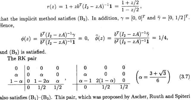
that the implicit method satisfies $(\mathrm{B}_{2})$. In addition, $\gamma=[0,0]^{T}$ and $\hat{\gamma}=[0,1/2]^{T}$.

Hence, $\phi(z)=\frac{b^{T}(I_{2}-zA)^{-1}\gamma}{b^{T}(I_{2}-zA)^{-1}1}=0$, $\hat{\phi}(z)=\frac{b^{T}(I_{2}-zA)^{-1}\hat{\gamma}}{b^{T}(I_{2}-zA)^{-1}1}=1/4$, and (B3) is satisfied. The RK pair

00000

0 0 $\alpha$ at 0 $\alpha$ 0 , $\alpha$ 0 0 $( \alpha=\frac{3+\sqrt{3}}{6})$ (3.7)

1 –at 0 $1-2\alpha$ $\alpha$ $\alpha-1$ $2(1-\alpha)$ 0

01/2 1/2 01/2 1/2 0 $\alpha$ 1 – $\alpha$ 0 0 0 0 $\alpha$ 0 0 1 - $2\alpha$ $\alpha$ 0 1/2 1/2 0 0 0 $\alpha$ 0 0 $\alpha-1$ $2(1-\alpha)$ 0 0 1/2 1/2

also satisfies $(\mathrm{B}_{1})$-(B3). This pair, whichwasproposed.byAscher, Ruuth and Spiteri

[2], determines athird order partitioned RK method for ODEs. In particular, $(\mathrm{B}_{1})$

is satisfied. The conditions $(\mathrm{B}_{2})$ and (B3) follow from

$(I_{3}-zA)^{-1}=[100$ $- \frac{()z}{(1-\alpha z)^{2}}\frac{01}{1-\alpha z,2\alpha-1}$, $\frac{001}{1-\alpha z}]$ ,

$zb^{T}(I_{3}-zA)^{-1}= \frac{z}{2}[0,$ $\frac{1-(3\alpha-1)z}{(1-\alpha z)^{2}}$, $\frac{1}{1-\alpha z}]$ ,

$r(z)= \frac{1-(2\alpha-1)z-(\alpha-1/3)z^{2}}{(1-\alpha z)^{2}}$,

$\phi(z)=(\frac{\alpha^{2}}{\underline{9}})\frac{(2\alpha-1)z}{2+(1-4\alpha)z}$ , $\hat{\phi}(z)=-\frac{\alpha^{2}(2\alpha-1)z}{2+(1-4\alpha)z}$

.

We apply the RK pairs (3.6) and (3.7) to the MOL approximation (3.4), and

integrate it from $t=0$ to $t=1$, with various gridsizes and stepsizes of the form

$\triangle t=h=\frac{1}{M}$ . (3.8)

Table 1shows the values

$-\log_{2}\epsilon_{M}$, $\epsilon_{M}=1\leq n\leq M\mathrm{m}\mathrm{a}\mathrm{x}(1\leq j\mathrm{m}\mathrm{a}\mathrm{x}\leq M|u(t_{n’ j}x)-u_{j}^{n}|)$ .

It is

observed

that $\epsilon_{M}$ is of$O(\Delta t^{2})$ for each method. Noting (3.5) and (3.8),

we

can

consider the result for (3.7) presents

an

order reduction phenomenon, i.e., the

error

ofa“third order” method behaves

as

$O(\Delta t^{2})$

.

(9)

Table 1. Numerical results for the model problem (3.1) (3.3) $\lambda l$ 20 40 80 160 320 640 Method (3.6) Method (3.7) 3.63 5.09 6.79 8.64 10.56 12.52 5.60 7.42 9.32 11.25 13.19 15.16

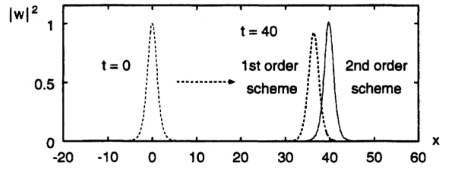
Fig. 1shows anumerical result concerning the “soliton solution”

$w(t,x)= \sqrt{2\alpha}\exp[\mathrm{i}\{\frac{c}{2}x-(\frac{c^{2}}{4}-\alpha)t\}]$ sech$[\alpha(x-ct)]$ (3.9)

to the simple nonlinear Schrodinger equation

$\frac{\partial w}{\partial t}=$ . $\frac{\partial^{2}w}{\partial x^{2}}+\cdot|w|^{2}w$

.

(3.10)

The ”1st order scheme” indicates the method (1.5), and the ”2nd order schem\"e’’

indicates the method (3.6). The values $\alpha=0.5$, _$c=1$, $\Delta x=0.2$, $\Delta t=0.005$

are

used for the computation.

$|\mathrm{w}|^{2}$ 1 $\mathrm{t}\mathrm{t}|||||_{1}|_{1}^{\backslash }$ $\mathrm{t}=40$ $\dot{\mathrm{i}}_{}^{}$ $\mathrm{t}\iota\iota^{\mathfrak{l}\mathrm{l}}\iota$

$\mathrm{t}=0$ $\mathrm{i}11$ 1storder $ii$ 2nd order

0.5 $|||||1||1|||!||-\cdot$ scheme $i_{1}^{1}\dot{\mathrm{i}}$ scheme $\prime\prime\prime \mathrm{l}.\iota^{t}1‘||\backslash .\backslash$

$\prime ^{\dot{}}$ $\dot{}_{1}$

0 $\mathrm{x}$ -20 -10 0 10 20 30 40 50 60 $\mathrm{t}\mathrm{t}|||||_{1}|_{1}^{\backslash }$ $\mathrm{t}=40$ $\dot{\mathrm{i}}_{}^{}$ $|\iota^{1}$ $\mathrm{l}\iota_{1}$

..

$\mathrm{t}=0$ $||\mathrm{i}$

$\mathrm{I}|1|-$

–\sim lst

order

$\mathrm{i}$ $i_{}$ 2nd order $\iota^{t}|||||1$ $1|!||1$ $-arrow$ _scheme $i$ $\overline{\mathrm{i}}$ scheme $\prime\prime\prime 1^{\cdot}$

$‘||\backslash .\backslash$ $’^{^{}}$ $\dot{}_{1}$

Fig. 1. Numerical solutions of the nonlinear Schrodinger equation (3.10).

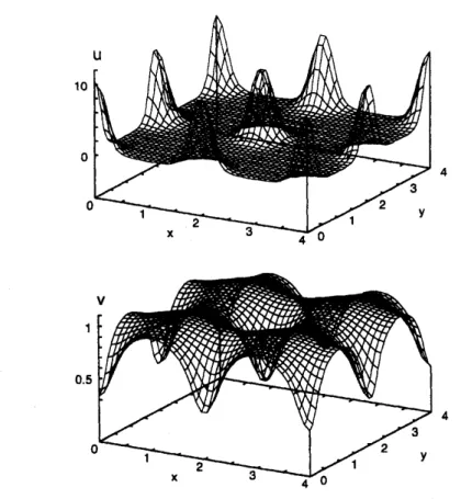
Fig. 2shows astationary solution to the equation (Brusselator)

$\{$

$\frac{\partial u}{\partial t}=D_{U}(\frac{\partial^{2}u}{\partial x^{2}}+\frac{\partial^{2}u}{\partial y^{2}})+\alpha-(\beta+1)u+u^{2}v$

$\frac{\partial v}{\partial t}=D_{V}(\frac{\partial^{2}v}{\partial x^{2}}+\frac{\partial^{2}v}{\partial y^{2}})+\beta u-u^{2}v$

(3.11)

$0\leq x\leq 4,0\leq y\leq 4$,

Du

$=0.02$,

Dv

$=1$,

cr

$=1$, $\beta=1.8$,

under the Neumann boundary condition, obtained by the method (3.6). These

figures suggest that the method (3.6) is useful for

some

problems

(10)

Fig. 2. Stationary solution to the equation (3.11).

References

[1] G. Akrivis, M. Crouzeix, C. Makridakis, Implicit-explicit multistep methods

for quasilinear parabolic equations, Numer. Math. 82 (1999), 521-541.

[2] U. M. Ascher, S. J. Ruuth, R. J. Spiteri, Implicit-explicit Runge-Kutta

meth-ods for time-dependent partial differential equations, Appl. Numer. Math. 25

(1997), 151-167.

[3] U. M. Ascher, S. J. Ruuth, B. T. R. Wetton, Implicit-explicit methods for

time-dependent partialdifferential equations, SIAM J. Numer. Anal. 32 (1995),

797-823.

[4] W. Bao,D. Jaksch, P. A. Markowich,

Numerical

solution of the

Gross-Pitaevskii

equation for Bose-Einstein condensation $(\mathrm{h}\mathrm{t}\mathrm{t}\mathrm{p}://\mathrm{b}\mathrm{o}\mathrm{z}\mathrm{o}\mathrm{n}.\mathrm{u}\mathrm{i}\mathrm{b}\mathrm{k}.\mathrm{a}\mathrm{c}.\mathrm{a}\mathrm{t}/\sim \mathrm{d}\mathrm{j}\mathrm{a}\mathrm{k}\mathrm{s}\mathrm{c}\mathrm{h})$ .

[5] K. Burrage, W. H. Hundsdorfer, J. G. Verwer, Astudy of $\mathrm{B}$

-convergence

of

Runge-Kutta methods, Computing, 36 (1986), 17-34.

[6] M. P. Calvo, J. de Frutos, J. Novo, Linearly implicit Runge-Kutta methods for

advection-reaction-diffusion

equations, Appl. Numer. Math. 37(2001), 535-549

(11)

[7] R. Frank, J. Schneid, C. W. Ueberhuber, The concept ofB convergence SIAM

J. Numer. Anal. 18 (1981), 753-780.

[8] D. F. Griffiths, A. R. Mitchell, J. $\mathrm{L}\mathrm{I}$. Morris, Anumericalstudy

of the nonlinear

Schrodinger equation, Comput. Methods Appl. Mech. Engrg. 45 (1984),

177-215.

[9] E. Hairer, S. P. NOrsett, G. Wanner, Solving Ordinary

_Differential

Equations $I$,

Nonstiff

Problems (2nd rev. ed.), Springer-Verlag, 1993.

[10] E. Hairer, G. Wanner, Solving Ordinary

_Differential

Equations

_If

_Stiff

and

Differential-Algebraic Problems (2nd rev. ed.), Springer-Verlag, 1996.

[11] D. Hoff, Stability and convergence of finite difference methods for systems of

nonlinear reaction-diffusionequations, SIAM J. Numer. Anal. 15 (1978), 1161

1177.

[12] K. J. in ’$\mathrm{t}$ Hout, On thecontractivityof implicit-explicit linear multistep

meth-ods Appl. Numer. Math. 42 (2002), 201-212.

[13] T. Koto, Explicit Runge-Kutta schemes for evolutionary problems in partial

differential equations, Ann. Numer. Math. 1(1994), 335-346.

[14] J. M. Sanz-Serna, J. G. Verwer, W. H. Hundsdorfer, Convergence and order

reduction of Runge-Kutta schemes applied to evolutional problems in partial

differential equations, Numer. Math. 50 (1986), 405-418.

[15] J. G. Verwer, Convergence and order reduction of diagonally implicit

Runge-Kutta schemes in the method of lines, in D. F. Griffiths, G. A. Watson (eds),

“Numerical analysis (Dundee, 1985)”, Pitman ${\rm Res}$

.

Notes Math. Ser. 140,

220-237, Longman

Scientific&Technical,

1986