A local analysis of the radial configuration for the two-phase torsion problem in the ball (Analysis on Shapes of Solutions to Partial Differential Equations)

全文

(1)7. 数理解析研究所講究録第2082巻 2018年 7-20. A local analysis of the radial configuration for the two‐phase torsion problem in the ball Lorenzo Cavallina. *. Abstract. This is a resume of [4]. We consider the configuration given by two concentric balls, made of different materials. We get precise information on the local opti‐ mality of this radially symmetric configuration for the two‐phase torsional rigidity functional under the effect of perturbations that act exclusively on the inner ball. while satisfy ing the volume (or surface area) preserving constraint. We perform shape derivatives up to the second order and make use of spherical harmonics to aid our calculations. Depending on the difference of the two conductivities, a symmetry breaking phenomenon occurs.. 2010 Mathematics Subject classification. 49\mathrm{Q}10. Keywords and phrases: torsion problem, optimization problem, elliptic PDE, shape demva‐ tive. Contents 1. 2. Introduction. 2. Computation of the first order shape derivative: Proof of Theorem 1.1. 3. 4. Computation of the second order shape derivative: Proof of Theorem 1.2. 4. 6. Some comments on the surface area preserving case. 11. ’This research was partially supported by the Grant‐in‐Aid for Scientific Research (B) (#26287020) Japan Society for the Promotion of Science. 1.

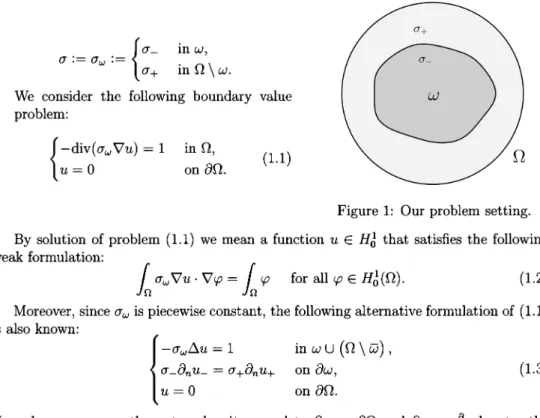
(2) 8. 1. Introduction. Let $\Omega$\subset \mathbb{R}^{N} (N\geq 2) be the unit open ball centred at the origin. Moreover, let $\omega$\subset\subset $\Omega$ be a sufficiently regular open set. Fix two positive constants $\sigma$_{-}, $\sigma$_{+} and consider the following distnbution of conductivities:. $\sigma$:=$\sigma$_{ $\omega$}:=. \left{bginary}{l $\sigma$_{-}&\mathr{i}\mathr{n}$\omega$,\ sigma$_{+}&\mathr{i}\mathr{n}$\Omega$\bckslah$\omega$. \end{ary}\ight.. We consider the following boundary value problem:. \left{\begin{ar y}{l -\mathrm{d}\mathrm{i}\ athrm{v}($\sigma$_{ \omega$}\nabl u)=1&\mathrm{i}\ athrm{n}$\Omega$,\ u=0&\mathrm{o}\mathrm{n}\partil$\Omega$. \end{ar y}\right.. (1.1) Figure 1: Our problem setting.. By solution of problem (1.1) we mean a function weak formulation:. Moreover, since. \displayst le\int_{$\Omega$} \sigma$_{$\omega$}\nablau\cdot\nabla$\varphi$=\int_{$\Omega$} \varphi$. $\sigma$_{ $\omega$}. u\in. H_{0}^{1} that satisfies the following. for all $\varphi$\in H_{0}^{1}( $\Omega$) .. (1.2). is piecewise constant, the following alternative formulation of (1.1). is also known:. \left{bginary}{l -$\sigma_{$\omega$}\tringleu=1&\mathr{i}\mathr{n}$\omega$\cup( Omega$\bckslah\overlin{$\omega$}),\ sigma$_{-}\prtial_{n}u-=$\sigma_{+}\prtial_{n}u+&on\partilw,\ u=0&\mathr{o}\mathr{n}\partil$\Omega$. \nd{ary}\ight.. (1.3). Here, by we mean the outward unit normal to \partial $\omega$ or \partial $\Omega$ and \partial_{n} := \displaytle\frac{\partil}{\partiln} denotes the usual normal derivative. Throughout the paper we will use \mathrm{t}\mathrm{h}\mathrm{e}+ and — subscripts to n. denote quantities in the two different phases. The second equality of (1.3), known in the literature as transmission condition, has to be intended in the sense of traces. In the sequel, the notation [f] :=f_{+}-f_{-} will be used to denote the jump of a function f through. the interface on. \partial $\omega$. (for example, the transmission condition can be written as [$\sigma$_{ $\omega$}\partial_{n}u]=0. \partial $\omega$. We aim to study the following torsional rigidity functional:. E($\omega$):=\displaystyle\int_{$\Omega$} \sigma$_{$\omega$}|\nablau_{$\omega$}|^{2}=$\sigma$_{-}\int_{$\omega$}|\nablau_{$\omega$}|^{2}+$\sigma$_{+}\int_{$\Omega$\backslash\overline{$\omega$}|\nablau_{$\omega$}|^{2} , where. u_{ $\omega$}. (1.4). is the unique solution of (1.1).. Physically speaking, the value E( $\omega$) represents the torsional rigidity of an infinitely long composite beam whose cross section is depicted in Figure 1. The values $\sigma$_{-}, $\sigma$+ , then, represent the hardness of the material of each phase. The study of similar energy functionals is not new. The onephase version of this prob‐. lem was first studied by Pólya in [17] by means of symmetric rearrangement inequalities. 2.

(3) 9. Pólya’s result tells us that homogeneous beams with a spherical section are the “most re‐. sistant” (precisely speaking, the ball maximises the one‐phase torsional rigidity functional among all Lipschitz domains of a fixed volume). Unfortunately, the technique employed by Pólya cannot be applied directly to a two‐phase setting because of the discontinuity of the coefficients. Inspired by the result of Pólya, we perform a local analysis of the. configuration given by. $\omega$. and. $\Omega$. being concentric balls. In [4], we study what happens to. the torsional rigidity after applying a small perturbation to the inner ball. We make use. of the shape derivative machinery that has been used by Conca and Mahadevan in [2], and Dambrine and Kateb in [6] for the minimisation of the first Dirichlet eigenvalue in a similar two‐phase setting ( $\Omega$ being a ball). In [5] we deal with more general perturbations: namely we allow pertubations that act on both \partial $\omega$ and \partial $\Omega$ simultaneously. This might give rise to some resonance effect that does not appear when \partial $\omega$ or \partial $\Omega$ are perturbed in isolation.. A direct calculation shows that the function u , solution to (1.3) where. $\omega$=. B_{R} , has. the following expression:. u(x)=. \{ \displayte\frac{ 1-R^{2} N$\sigma$_{\dager$}1-|x^{2} N$\sigma$+}\frac{R^2}-|x{}2N$\sigma$-}. for. |x|. \in[0, R],. (1.5). for |x| \in[R , 1 ].. In this paper we will use the following notation for Jacobian and Hessian matrix respec‐ tively.. (Dv)_{ij}:=\displaystyle \frac{\partial v_{i} {\partial x_{j} , (D^{2}f)_{ij}=\frac{\partial^{2}f {\partial x_{i}\partial x_{j} ,. f and vector field v=(v_{1}, \ldots, v_{N}) defined on $\Omega$ . We will introduce some differential operators from tangential calculus that will be used in the sequel. For smooth f and v defined on \partial $\omega$ we set for all smooth real valued function. \nabla_{ $\tau$}f. :=\nabla\overline{f}-(\nabla\tilde{f}\cdot n)n. (tangential gradient), (tangential divergence),. \mathrm{d}\mathrm{i}\mathrm{v}_{ $\tau$}v :=\mathrm{d}\mathrm{i}\mathrm{v}\overline{v}-n\cdot(D\overline{v}n). where. \tilde{f} and \tilde{v} are some. smooth extensions on the whole. $\Omega$. of f and. v. (1.6) respectively. It is. known that the differential operators defined in (1.6) do not depend on the choice of the extensions. Moreover we let D_{ $\tau$}v denote the matrix whose i‐th row is given by \nabla_{ $\tau$}v_{i} . We. define the (additive) mean curvature of. \partial $\omega$ as H :=\mathrm{d}\mathrm{i}\mathrm{v}_{ $\tau$}n (cf. [8, 12 \parti a l B_{R} of is given by (N-1)/R.. According to this. definition, the mean curvature A first key result of this paper is the following. H. Theorem 1.1. For all suitable perturbations that fix the volume, the first order shape derivative of E at B_{R} vanishes. Actually, Theorem 1.1 holds true under the weaker assumption that our perturbation. satisfies the first order volume preserving condition (2.11). An improvement of Theorem 1.1 is given by the following precise result (obtained by studying second order shape derivatives).. 3.

(4) 10. Theorem 1.2. Let $\sigma$_{-}, $\sigma$_{+} >0 and R\in (0,1) . If $\sigma$_{-} > $\sigma$+ then B_{R} is a local maximiser for the functional E under the fixed volume constraint. On the other hand, if $\sigma$_{-} <$\sigma$_{+} then B_{R} is a saddle shape for the functional E under the fixed volume constraint.. This work is organised as follows: in section 2 the concept of shape derivative is introduced and results concerning the first order shape derivative of the functional E are presented. In section 3 we deal with the second order shape derivative of the functional E and the study of its sign by means of a spherical harmonic expansion. In section 4 we examine the differences that arise when we replace the volume constraint with a surface area one.. 2. Computation of the first order shape derivative: Proof of Theorem 1.1. We consider the following class of perturbations that act on B_{R} without altering \partial $\Omega$ :. \mathcal{A}:=\{ $\Phi$\in C^{\infty}([0,1)\times \mathb {R}^{N}, \mathb {R}^{N}) | $\Phi$(t,x)=x\mathrm{f}\mathrm{o}\mathrm{r}t\in[0,1),|x\geq R_{0} $\Phi$(0,\cdot)=\mathrm{I}\mathrm{d},\suchthat exist R_{0}\in(R,1) }. (2.7) For $\Phi$\in \mathcal{A} we will write $\Phi$(t) to denote $\Phi$(t, \cdot) and, for all domain D in \mathbb{R}^{N}, $\Phi$(t)(D) will denote the set of all $\Phi$(t, x) for x \in D . In the sequel the following notation for the. first order approximation (in the ( time” variable) of $\Phi$(t)=\mathrm{I}\mathrm{d}+th+o(t). as. $\Phi$. will be used:. for some smooth h:\mathbb{R}^{N}\rightarrow \mathbb{R}^{N} .. t\rightarrow 0 ,. (2.8). In particular it will be useful to separate the normal and tangential component of h : we write h_{n} :=h\cdot n and h_{ $\tau$} :=h-h_{n}n on \partial B_{R} . We define the shape derivative of a shape functional J with respect to a deformation field $\Phi$ in \mathcal{A} as follows:. \displaystyle \frac{d}{dt}J( $\Phi$(t)(D) |_{t=0}=\lim_{t\rightar ow 0}\frac{J( $\Phi$(t)(D) -J(D)}{t}. This subject is very deep. Many different formulations of shape derivatives associated. to various kinds of deformation fields have been proposed over the years. We refer to [8] for a detailed analysis on the equivalence between the various methods. For the study. of second (or even higher) order shape derivatives and their computation we refer to [8, 13, 16, 18]. The structure theorem for first and second order shape derivatives (cf. [12, Theorem 5.9.2, page 220] and the subsequent corollaries) yields the following expansion. For every shape functional J , domain D and pertubation field assumptions the following holds:. J( $\Phi$(t)(D)). $\Phi$. in \mathcal{A} , under suitable smoothness. =J(D)+tl_{1}^{J}(D)(h_{n})+\displaystyle \frac{t^{2} {2}(l_{2}^{J}(D)(h_{n}, h_{n})+l_{1}^{J}(D)(Z) +o(t^{2}) as. for some linear. l_{1}^{J}(D) : C^{\infty}(\partial D). \rightar ow \mathbb{R} and bilinear form. (2.9). l_{2}^{J}(D) : C^{\infty}(\partial D)\times C^{\infty}(\partial D)\rightarrow \mathbb{R}. to be determined eventually. Moreover for the ease of notation we have set. Z := (V'+Dhh)\cdot n+((D_{ $\tau$}n)h_{ $\tau$})\cdot h_{ $\tau$}-2\nabla_{ $\tau$}h_{n}\cdot h_{ $\tau$}, 4. t\rightarrow 0 ,.

(5) 11. where V(t, $\Phi$(t)) :=\partial_{t} $\Phi$(t) and V' :=\partial_{t}V(t ,. on the boundary of. D. Perturbations of the form $\Phi$=\mathrm{I}\mathrm{d}+th_{n}n. are usually called Hadamard perturbation. As (2.9) shows, using. only Hadamard perturbations is enough to compute the first order shape derivative of. a functional (and also the bilinear part of its second order shape derivative l_{2}^{J} for that matter). On the other hand, second order derivatives contain an extra term l_{1}^{J}(D)(Z) that depends on higher terms of the expansion of $\Phi$ . It is woth noticing that, (see [12, Corollary 5.9.4, page 221]) Z vanishes in the special case when $\Phi$ is a Hadamard perturbation (this is a key observation, crucial to the computation of the bilinear form l_{2}^{J} in [4, Theorem 3.1]). We introduce the class of perturbations in \mathcal{A} that fix the volume of B_{R} : \mathcal{B}. :=\{ $\Phi$\in \mathcal{A}|\mathrm{V}\mathrm{o}\mathrm{l}( $\Phi$(t)(B_{R}) =\mathrm{V}\mathrm{o}\mathrm{l}(B_{R}). for all t\in[0 , 1. The following expansion is also well known. For all $\Phi$\in \mathcal{A} we have. \displaystyle\mathrm{V}\mathrm{o}\mathrm{l}($\Phi$_{t}(B_{R}) =\mathrm{V}\mathrm{o}\mathrm{l}(B_{R})+t\int_{\partialB_{R} h_{n}+\frac{t^{2} {2} (\displaystyle \int_{\partial B_{R} Hh_{n}^{2}+\int_{\partial B_{R} Z)+o(t^{2}) as. t\rightarrow 0 .. (2.10). This yields the following two volume preserving conditions:. \displaystyle \int_{\partial B_{R} h_{n}=0, \displaystyle \int_{\partial B_{R} Hh_{n}^{2}+\int_{\partial B_{R} Z=0.. ( 1^{\mathrm{s}\mathrm{t} order volume preserving). (2.11). ( 2^{\mathrm{n}\mathrm{d} order volume preserving). (2.12). Notice that condition (2.12) implies that Hadamard perturbations cannot be volume pre‐ serving (that is one of the reasons why whe had to include more general perturbations in the definition of \mathcal{A} , (2.7)). Usually, shape functionals can also depend on the domain indirectly, by means of some functions defined on it, those are called state functions in literature. In our case,. the function u_{ $\omega$} , solution of problem (1.1) is the only state function for the functional E defined in (1.4). We will now introduce the concepts of“shape” and “material”’ derivative of a state function defined on. $\Omega$ .. u=u(t, x) be defined on [0 , 1). \times $\Omega$ .. Fix an admissible perturbation field. $\Phi$ \in A. and let. Computing the partial derivative with respect to. at a fixed point x\in $\Omega$ is usually called shape derivative of. u'(t_{0}, x):=\displaystyle \frac{\partial u}{\partial t}(t_{0}, x) ,. u. t. ; we will write:. for x\in $\Omega$, t_{0}\in[0 , 1).. On the other hand differentiating along the trajectories gives rise to the material denva‐ tive:. \displaystyle \dot{u}(t_{0}, x) :=\frac{\partial v}{\partial t}(t_{0}, x) , x\in $\Omega$, t_{0}\in[0, 1). ;. where v(t, x) := u(t, $\Phi$(t, x From now on for the sake of brevity we will omit the dependency on the time” variable and write u(x), u'(x) and \dot{u}(x) for u(0, x), u'(0, x) and \dot{u}(0, x) . The following relationship between shape and material derivatives hold true: (. u'=\dot{u}-\nabla u\cdot h 5. (2.13).

(6) 12. In the case where u(t, \cdot) := u_{ $\Phi$(t)(B_{R})} (i.e. it is the solution to problem (1.1) when $\Phi$(t)(B_{R})) , by symmetry, we have: u'=\dot{u}-(\partial_{n}u)h_{n}. on \partial B_{R} .. In accordance with the classical theory (see for example [16]), for. $\omega$. =. (2.14) k\in \mathbb{N} ,. the k‐th order. shape derivative of an integral functional depends on the (k-1)-\mathrm{s}\mathrm{t} shape derivative of its state functions. Therefore we need only compute u' . We give the following characterisation. (see [4, Proposition 2.3]): Proposition 2.1. For any given admissible $\Phi$\in \mathcal{A} , the corresponding u' can be charac‐. terised as the (unique) solution to the following problem in the class of functions that are smooth in the open set. B_{R}\cup( $\Omega$\backslash \overline{B_{R} ) :. \left{bginary}{l $\Deltau'=0&inB_{R}\cup($Omega$\bckslah\overlin{B_R}),\ {[$sigma\prtil_{n}u']=0&on\partilB_{R},\ [u']=-\partil_{n}u]h &on\partilB_{R},\ u'=0&on\partil$\Omega$. \nd{ary}\ight.. (2.15). As usual when dealing with perturbations that act on the interface of discontinuity. of the coefficients, the Hadamard’s formulas cannot be applied directly (we refer to [12, formula (5.17) page 176 and formulas (5.110)‐(5.111) page 227] for a proof of those useful formulas in the smooth one‐phase setting). Instead, we have to split the integral as done in (1.4) and apply the Hadamard’s formula to each integral (this is a standard procedure, followed for example by [2,6], among many others). This gives rise to surface integrals on the interface as shown in the following theorem. We refer to [4, Theorem 2.4] for a proof. Theorem 2.2. For all $\Phi$\in \mathcal{A} we have. l_{1}^{E}(B_{R})(h_{n})=-\displaystyle \int_{\partial B_{R} [ $\sigma$|\nabla u|^{2}]h_{n}. In particular, by symmetw, for all. (2.11) (and thus for all. 3. $\Phi$\in \mathcal{B} ). $\Phi$. satisfying the first order volume preserving condition. we get l_{1}^{E}(B_{R})(h_{n})=0.. Computation of the second order shape derivative: Proof of Theorem 1.2. The result of the previous chapter tells us that the configuration corresponding to B_{R} is a critical shape for the functional E under the fixed volume constraint. In order to obtain more precise information, we will need an explicit formula for the second order shape derivative of E . The first step consists of the computation of the bilinear form. l_{2}^{E}(B_{R})(h_{n}, h_{n}) (we refer to [4, Theorem 3.1] for the proof).. Theorem 3.1. For all $\Phi$\in \mathcal{A} we have. l_{2}^{E}(B_{R})(h_{n}h_{n})=-2\displaystyle \int_{\partial B_{R} $\sigma$_{-}\partial_{n}u_{-} [\displaystyle \partial_{n}u']h_{n}-2\int_{\partial B_{R} $\sigma$_{-}\partial_{n}u_{-}[\partial_{n }^{2}u]h_{n}^{2}-\int_{\partial B_{R} $\sigma$_{-}\partial_{n}u_{-}[\partial_{n}u]Hh_{n}^{2}. 6.

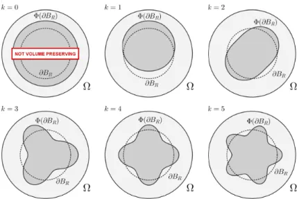
(7) 13. By Theorem(2.2), for all. $\Phi$\in \mathcal{B}. and. t>0. small, the expansion (2.9) corresponding to. the functional E reads. E( $\Phi$(t)(B_{R})). =E(B_{R})+\displaystyle \frac{t^{2} {2} (l_{2}^{E}(B_{R})(h_{n}h_{n})-\displaystyle \int_{\partial B_{R} [ $\sigma$|\nabla u|^{2}]Z)+o(t^{2}) as. t\rightarrow 0 .. (3.16). Employing the use of the second order volume preserving condition (2.12) and the fact that, by symmetry, the quantity. [ $\sigma$|\nabla u|^{2}]. is constant on the interface \partial B_{R} we have. -\displaystyle \int_{\partial B_{R} [ $\sigma$|\nabla u|^{2}]Z=\int_{\partial B_{R} [ $\sigma$|\nabla u|^{2}]Hh_{n}^{2}. Combining this with the result of Theorem 3.1 yields. E( $\Phi$(t)(B_{R})). =E(B_{R})+t^{2}\displaystyle \{-\int_{\partial B_{R} $\sigma$_{-}\partial_{n}u_{-}[\partial_{n}u']h_{n}-\int_{\partial B_{R} $\sigma$_{-}\partial_{n}u_{-}[\partial_{n }^{2}u]h_{n}^{2}\}+o(t^{2}). .. We will denote the expression between braces in the above by Q(h_{n}) . Since u' depends linearly on h_{n} (see (2.15)), it follows immediately that Q(h_{n}) is a quadratic form in h_{n}.. Some elementary calculation involving (1.5) and (2.15) yields. Q(h_{n})=\displaystyle\frac{R}{N}(\frac{1}{$\sigma$_{-} \frac{1}{$\sigma$_{+} )(-\int_{\partialB_{R} $\sigma$_{-}\partial_{n}u_{-}h_{n}+\frac{1}{N}\int_{\partialB_{R} h_{n}^{2}). (3.17). In the following we will try to find an explicit expression for u' . To this end we will perform the spherical harmonic expansion of the function h_{n} : \partial B_{R}\rightarrow \mathbb{R} . We set. h_{n}(R$\theta$)=\displaystyle\sum_{k=1}^{\infty}\sum_{i=1}^{d_{k}$\alpha$_{k,i}Y_{k,i}($\theta$). for all $\theta$\in\partial B_{1} .. (3.18). The functions Y_{k,i} are called sphencal harmonics in the literature. They form a complete orthonormal system of L^{2}(\partial B_{1}) and are defined as the solutions of the following eigenvalue problem: -\triangle_{ $\tau$}\mathrm{Y}_{k,i}=$\lambda$_{k}Y_{k,i} on \partial B_{1}, where \triangle_{ $\tau$} :=\mathrm{d}\mathrm{i}\mathrm{v}_{ $\tau$}\nabla_{7} is the Laplace‐Beltrami operator on the unit sphere. We impose the following normalisation condition. \displaystyle \int_{\partial B_{1} Y_{k,i}^{2}=R^{1-N} .. (3.19). The following expressions for the eigenvalues $\lambda$_{k} and the corresponding multiplicities d_{k}. are also known (for some reason, the expression for d_{k} appearing in [4, (4.26)] is wrong):. $\lambda$_{k}=k(k+N-2) , d_{k}=\displaystyle \frac{(2k+N-2)(k+N-3)!}{k!(N-2)!} .. (3.20). Notice that the value k=0 has to be excluded from the summation in (3.18) because we require h_{n} to verify the first order volume preserving condition (2.11) (also look at Figure 2 to get the gist of how perturbations related to different values of k work). 7.

(8) 14. k=0. Figure 2: How $\Phi$(t)(B_{R}) looks like for small. t. when h_{n}(R\cdot)=Y_{k,i} , in 2 dimensions.. Let us pick an arbitrary k\in\{1 , 2, . . . \} and i\in\{1, . . . , d_{k}\} . We will use the method of separation of variables to find the solution of problem (2.15) in the particular case when h_{n}(R $\theta$)=Y_{k,i}( $\theta$) , for all $\theta$\in\partial B_{1} and then the general case will be recovered by linearity.. r. We will be searching for solutions to (2.15) of the form u'=u'(r, $\theta$)=f(r)g( $\theta$) (where :=|x| and $\theta$ :=x/|x| for x\neq 0 ). Using the well known decomposition formula for the. Laplacian into its radial and angular components, the equation \triangle u'=0 in. B_{R}\cup( $\Omega$\backslash \overline{B_{R} ). can be rewritten as. 0=\displaystyle \triangle u'(x)=f_{r }(r)g( $\theta$)+\frac{N-1}{r}f_{r}(r)g( $\theta$)+\frac{1}{r^{2} f(r)\triangle_{ $\tau$}g( $\theta$) for r\in(0, R)\cup(R, 1) , $\theta$\in\partial B_{1}. Take g=Y_{k,i} . Under this assumption, we get the following equation for f :. f_{r }+\displaystyle \frac{N-1}{r}f_{r}-\frac{$\lambda$_{k} {r^{2} f=0. in (0, R)\cup(R, 1) .. (3.21). It can be easily checked that, on each interval (0, R) and (R, 1) , any solution to the above consists of a linear combination of the following two independent solutions:. f_{sing}(r):=r^{2-N-k} Since equation (3.21) is defined for. r\in. and. f_{reg}(r):=r^{k} .. (3.22). (0, R)\cup(R, 1) , we have that the following holds. for some real constants A_{k}, B_{k}, C_{k} and D_{k} ;. f(r)=. \left\{ begin{ar y}{l A_{k}r^{2-Nk}+B_{k}r^{k}\mathrm{f}\mathrm{o}\mathrm{}r\in(0,R),\ C_{k}r^{2-Nk}+D_{k}r^{k}\mathrm{f}\mathrm{o}\mathrm{}r\in(R,1). \end{ar y}\right.. Moreover, since 2-N-k is negative, A_{k} must vanish, otherwise a singularity would occur at r=0 . The other three constants can be obtained by the interface and boundary 8.

(9) 15. conditions of problem (2.15) bearing in mind that u'(r, $\theta$). =. f(r)Y_{k,i}( $\theta$). =. f(r)h_{n}(R $\theta$) .. We get the following system:. \left{\begin{ar y}{l C_{k}R^{2-Nk}+D_{k}R^{k}-B_{k}R^{k}=-\frac{R}N$\sigma$-}+\frac{R}N$\sigma$+},\ $\sigma$_{-}kB_{}R^{k-1}=$\sigma$_{+}(2-Nk)C_{k}R^{2-Nk}+$\sigma$_{+}kD_{}R^{k-1},\ C_{k}+D_{k}=0. \end{ar y}\right.. We solve the system above for B_{k} :. B_{k}=\displaystyle\frac{R^{1-k} {N$\sigma$_{-} \cdot\frac{k($\sigma$_{-}$\sigma$_{+})-(2-N-k)($\sigma$_{-}$\sigma$_{+})R^{2-N-2k} {k($\sigma$_{-}$\sigma$_{+})+( 2-N-k)$\sigma$_{+}-k$\sigma$_{-})R^{2-N-2k} .. (3.23). Therefore, in the particular case when h_{n}(R\cdot)=Y_{k,i} we obtain u. ’‐. =u_{-}'(r, $\theta$)=B_{k}r^{k}Y_{k,i}( $\theta$) ,. r\in[0, R) ,. $\theta$\in\partial B_{1}.. By linearity, we recover the expansion of u' ‐in the general case (i.e. when (3.18) holds):. u_{-}'(r, $\theta$)=\displaystyle\sum_{k=1}^{\infty}\sum_{i=1}^{d_{k}$\alpha$_{k}B_{k}r^{k}\mathrm{Y}_{k,i}($\theta$) r\in[0, R) \displaystyle\partial_{n}u_{-}'(R, $\theta$)=\sum_{k=1}^{\infty}\sum_{i=1}^{d_{k} $\alpha$_{k}B_{k} R^{k-1}Y_{k,i}($\theta$) ,. ,. , $\theta$\in\partial B_{1} ,. and therefore. (3.24) $\theta$\in\partial B_{1}.. We can now diagonalise the quadratic form Q in (3.17). In other words we can consider only the case h_{n}(R\cdot) =Y_{k,i} for all possible pairs (k, i) . Actually, the dependence on the parameter. i. can be removed: without loss of generality we can consider Q as a function. of k as follows:. Q(h_{n})=Q(k, i)=Q(k)=\displaystyle \frac{R}{N}(\frac{$\sigma$_{+}-$\sigma$_{-} {$\sigma$_{+}$\sigma$_{-} ) (-$\sigma$_{-}B_{k}kR^{k-1}+\frac{1}{N}) = \displayst le\frac{R}N^{2}(\frac{$\sigma$_{+}-$\sigma$_{-} $\sigma$_{+}$\sigma$_{-}) \displaystyle \{1-k\frac{k($\sigma$_{-} $\sigma$_{+})+(N-2+k)($\sigma$_{-} $\sigma$_{+})R^{2-N-2k} {$\sigma$_{-}k(1-R^{2-N-2k})+$\sigma$_{+}(k+(2-N-k)R^{2-N-2k}) \}.. (3.25). Notice that the denominator in the expression in braces above is always negative for N\geq 2, k\geq 1 and R\in(0,1) : as a consequence, Q(k) is well defined.. Q(k) holds true for all k \geq Remark 3.2. The fact that, as shown in (3.25), Q(k, i) 1 and i \in \{1, . . . , d_{k}\} (i.e . the “oreentation” of the perturbation is not relevant) is a =. consequence of the radial symmetry of the configuration that we are studying and of the rotational invariance of the functional E. On the other hand, when both \partial B_{R} and \partial $\Omega$ are. perturbed simultaneously, as done in [5], the rotational symmetw is lost and the parameter i must also be taken into account.. We are now ready to prove the main result of the paper.. 9.

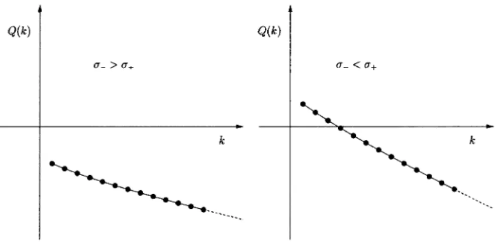
(10) 16. Theorem 3.3. Let. $\sigma$_{-}, $\sigma$_{+} >0. and R\in(0,1) . If $\sigma$_{-} >$\sigma$_{+} then. \displaystyle \frac{d^{2} {dt^{2} E( $\Phi$(t)(B_{R}) |_{t=0}<0. for all $\Phi$\in \mathcal{B}.. Hence, B_{R} is a local maximiser for the fUnctional E under the fixed volume constraint. On the other hand, if $\sigma$_{-}<$\sigma$_{+} , then there exist some $\Phi$_{1} and $\Phi$_{2} in \mathcal{B} , such that. \displaystyle \frac{d^{2} {dt^{2} E($\Phi$_{1}(t)(B_{R}) |_{t=0}<0, \frac{d^{2} {dt^{2} E($\Phi$_{2}(t)(B_{R}) |_{t=0}>0. In other words, B_{R} is a saddle shape for the functional. E. under the fixed volume con‐. straint.. Figure 3: The graph of Q(k) when. $\sigma$_{-}> $\sigma$+. (left) and when. $\sigma$_{-}. <$\sigma$_{+}. (right).. Proof. We will rewrite (3.25) more compactly as follows:. Q(k)=\displaystyle\frac{R}{N^{2} (\frac{$\sigma$_{+}-$\sigma$_{-} {$\sigma$_{+}$\sigma$_{-} )(1-k\frac{\mathcal{N} {\mathcal{D} ) First, suppose that. $\sigma$_{-}. > $\sigma$+\cdot. .. As remarked after (3.25), the denominator. moreover, since by hypothesis $\sigma$_{-} > $\sigma$+ , we also have \mathcal{N}> negative for all k\geq 1 , and hence. \displaystyle \frac{d^{2} {dt^{2} E( $\Phi$(t)(B_{R}) |_{\mathrm{t}=0}<0. for all. 0.. \mathcal{D}. is negative;. This implies that Q(k) is. $\Phi$\in \mathcal{B},. as claimed.. Now suppose that. $\sigma$_{-}. < $\sigma$+\cdot We have >0 .. Q(1)=. 10. (3.26).

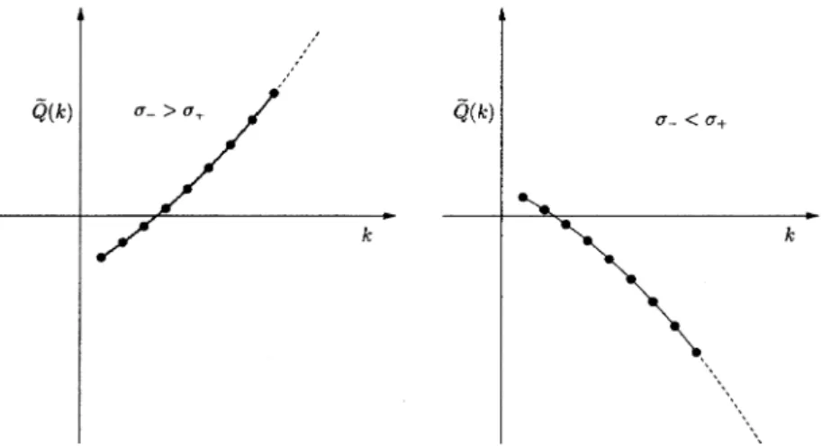
(11) 17. On the other hand, an elementary calculation shows that (actually for all. \displaystyle \lim_{k\rightar ow\infty}Q(k)=-\infty . Combining (3.26) and (3.27) we get that, when. $\sigma$_{-}. $\sigma$_{-},. $\sigma$_{+}>0 ). (3.27) < $\sigma$+,. B_{R} is a saddle shape for the. functional E under the fixed volume constraint.. \square. As Figure 3 suggests, the function k\mapsto Q(k) is actually strictly decreasing. This is. proven in [4 Lemma 4.1] by treating derivative. 4. \displaystyle \frac{d}{dk},Q(k). k. as a real variable and studying the sign of the. .. Some comments on the surface area preserving case. The method employed in this paper can be applied to other geometrical constraints as well. In particular we studied what happens when volume preserving perturbations are replaced by surface area preserving ones. We need to replace (2.11)-(2.12) by the following well known first and second order. surface area preserving conditions (see for instance [12, page 225. \displaystyle \int_{\partial B_{R} Hh_{n}=0, \displaystyle \int_{\partial B_{R} |\nabla_{ $\tau$}h_{n}|^{2}+\int_{\partial B_{R} (H^{2}-\mathrm{t}\mathrm{r}( D_{ $\tau$}n)^{T}D_{ $\tau$}n) h_{n}^{2}+\int_{\partial B_{R}(4.28) HZ=0. Notice that, as. H. is constant on B_{R} , the first equality in (4.28) is equivalent to (2.11). and hence, the result of Theorem 2.2 holds true for surface area preserving perturbations as well.. The study of the second order shape derivative of. E. under this constraint is done as. before by replacing (2.12) by the second equation in (4.28). We are able to write the shape Hessian of E as a quadratic form in h_{n} . It can be then diagonalised by considering h_{n}(R\cdot) \mathrm{Y}_{k,i} for all possible pairs (k, i) , under the normalisation (3.19). Under this =. assumption, by (3.20) we get. \displaystyle \int_{\partial B_{R} |\nabla_{ $\tau$}h_{n}|^{2}=\frac{$\lambda$_{k} {R^{2} =\frac{k(k+N-2)}{R^{2} . We obtain. E( $\Phi$(t)(B_{R})) =E(B_{R})+t^{2}\overline{Q}(k)+o(t^{2}) where. \tilde{Q}(k). as. t\rightarrow 0,. is given by the following:. \displayst le\frac{R}N^{2}(\frac{$\sigma$_{+}-$\sigma$_{-} $\sigma$_{+}$\sigma$_{-}) (\displaystyle \frac{3}{2}-\frac{k(k+N-2)}{2(N-1)}-k\frac{k($\sigma$_{-} $\sigma$_{+})-(2-N-k)($\sigma$_{-} $\sigma$_{+})R^{2-N-2k} {k($\sigma$_{-} $\sigma$_{+})+( 2-N-k)$\sigma$_{+}-k$\sigma$_{-})R^{2-N-2k} ) It is immediate to check that \overline{Q}(1) Q(1) and therefore, \overline{Q}(1) is negative for $\sigma$_{-} > \infty for $\sigma$_{-} > $\sigma$+ and $\sigma$_{+} and positive otherwise. On the other hand, \displaystyle \lim_{k\rightar ow\infty}\overline{Q}(k) -\infty for $\sigma$_{-} < $\sigma$_{+} . In other words, under the surface area preserving \displaystyle \lim_{k\rightar ow\infty}\overline{Q}(k) constraint, B_{R} is always a saddle shape, independently of the relation between $\sigma$_{-} and =. =. =. 11. ..

(12) 18. Figure 4: The graph of \overline{Q}(k) when. $\sigma$_{-}>$\sigma$_{+}. (left) and when. $\sigma$_{-}. <$\sigma$_{+}. (right).. $\sigma$+\cdot This result has the following intuitive geometric interpretation. Since the case k=1 corresponds to deformations that coincide with translations at first order, it is natural to expect a similar behaviour under both volume and surface area preserving constraint. On. the other hand, high frequency perturbations (i.e. those corresponding to a very large eigenvalue) lead to the formation of indentations in the surface of B_{R} as shown in Figure 2. Hence, in order to prevent the surface area of B_{R} from expanding, its volume must inevitably shrink. This behaviour is shown in Figure 5. Together with the number of “indentations”, this shrinking effect must become stronger the larger k is, this suggests that the behaviour of E( $\Phi$(t)(B_{R})) for large k might be approximated by that of the. extreme case. $\omega$=\emptyset.. (. Figure 5: Under the surface area preserving constraint, $\Phi$(B_{R}) progressively shrinks” as k. gets larger and larger (here. k=14 ).. 12.

(13) 19. References [1] L. Ambrosio, G. Buttazzo, An optimal design problem with perimeter penalization, Calc. Var. Part. Diff. Eq. 1 (1993): 55‐69. [2] C. Conca, R. Mahadevan, L.Sanz, Shape demvative for a two‐phase eigenvalue prob‐ lem and optimal configuration in a ball. In CANUM 2008, ESAIM Proceedings 27,. EDP Sci., Les Ulis, France, (2009): 311‐321. [3] C. Bandle, A. Wagner, Second domain vareation for problems with Robin boundary conditions. J. Optim. Theory Appl. 167 (2015), no. 2: 430‐463.. [4] L. Cavallina, Locally optimal configurations for the two‐phase torsion problem in the ball. Nonlinear Anal., 162, (2017) 33‐48. [5] L. Cavallina, On the stability of the radially symmetric configuration for the two‐phase torsion problem under general perturbations. (in preparation). [6] M. Dambrine, D. Kateb, On the shape sensitivity of the first Dirichlet eigenvalue for two‐phase problems. Applied Mathematics and optimization 63.1 (Feb 2011): 45‐74.. [7] M. Dambrine, J. Lamboley, Stability in shape optimization with second variation. arXiv: 1410. 2586vl [math.OC] (9 Oct 2014). [8] M.C. Delfour, Z.‐P. Zolésio, Shapes and Geometrees: Analysis, Differential Calculus, and optimization. SIAM, Philadelphia (2001).. [9] G. De Philippis, A. Figalli, A note on the dimension of the singular set in free interface problems, Differential Integral Equations Volume 28, Number 5/6 (2015): 523‐536.. [10] L. Esposito, N. Fusco, A remark on a free interface problem with volume constraint, J. Convex Anal. 18 (2011): 417‐426.. [11] D. Gilbarg, N.S. Trudinger, Elliptic Partial Differential Equation of Second Order, second edition, Springer.. [12] A. Henrot, M. Pierre, Variation et optimisation de formes. Mathématiques& Appli‐ cations. Springer Verlag, Berhn (2005). [13] R. Hiptmair, J. Li, Shape derevatives in differential forms I: an intrinsic perspective, Ann. Mate. Pura Appl. 192(6) (2013): 1077‐1098. [14] C.J. Larsen, Regularity of components in optimal design problems with perimeter penalization, Calc. Var. Part. Diff. Eq. 16 (2003): 17‐29.. [15]. $\Gamma$.\mathrm{H} .. Lin, Variational problems with free interfaces, Calc. Var. Part. Diff. Eq. 1 (1993):149‐168.. [16] A. Novruzi, M. Pierre, Structure of shape derivatives. Journal of Evolution Equations 2 (2002): 365‐382. 13.

(14) 20. [17] G. Pólya, Torsional rigidity, principal frequency, electrostatic capacity and sym‐ metnzation. Q. Appl. Math. 6 (1948): 267‐277. [18] J. Simon, Second vanations for domain optimization problems, International Series of Numerical Mathematics, vol. 91. Birkhauser, Basel (1989): 361‐378. RESEARCH CENTER FOR PURE AND APPLIED MATHEMATICS, GRADUATE SCHOOL OF INFORMATION SCIENCES, TOHOKU UNIVERSITY, SENDAI 980‐8579 , JAPAN. Electronic mail address: [email protected]. $\iota$. 14.

(15)