Article
Time-Series Multivariate Analysis
by Orbit Analysis and Principal Component Analysis
Combined (1)
1 )ITAKI,
Masahiko
Contents
Introduction
Ⅰ.Partial correction of orbit analysis
Ⅱ.Some features of principal component analysis Ⅲ.Analysis of Japan s GDP
(1)Basic analysis (2)Orbit analysis
(3)Principal component analysis 1.Terms
2.Interpretation
(4)Developmental principal component analysis (The following is in the next issue.) 1.Two-principal-component analysis: extraction of basic opposing relations 2.Three-principal-component analysis: extraction of developed opposing relations 3. Four-principal-component analysis: extraction of opposing relations in totality
(a hierarchy of opposing relations)
(5)Principal component analysis and orbit analysis combined 1.Multiple regression analysis of principal components
2. The multiplier effect measured by multiple regression analysis of principal components
3.Orbit analysis of principal components
4.Orbit analysis of variables and principal components: extraction of causality
Key words : GDP, Multiplier effect, Orbit analysis, Developmental principal component
analysis, Multiple regression analysis of principal components, Orbit analysis of variables and principal components, Causality
Introduction
Either in natural science or social science, the fundamental purpose of research is to understand changes of an object over time on the basis of its structural analysis. For that
purpose scientists devise diverse variables and observe their variations. However, those variables which are hypothetically chosen for the sake of measurement of variations rarely represent the actual substance of the object or forces that bring about its changes. We could expect much less to identify clear causality among those variables.
It is the case for aggregates of GDP that are taken as an example in the present article: a bit surprising as it may sound to the common sense of Keynesian economics, those aggregates, i.e. fixed capital formation, household consumption, trade balance and government consumption, are all variables for observing and measuring a national economy, rather than its substance or driving forces per se. In order to understand this point, let us take an example of school examinations of five subjects, i.e. literature, mathematics, natural science, social science and English. Although they are five subjects for educating students or variables for measuring their academic achievements, intrinsic academic capabilities can be more properly explained by certain synthetic variables independent from each other, such as general academic ability , natural-science-biased ability and humanities-biased ability . This is the basic idea by which principal component analysis is conducted.
The purpose of this article is, as already suggested above, to examine the question of What is the unit of change? The unit can be understood as substance of a research object or a force that brings about changes, which we analyze on the basis of ordinary principal component analysis. It is followed by developmental principal component analysis in order to elucidate multilayered structure of forces that bring about changes , in which orthogonal principal components are dialectically interpreted as multilayered structure of unified opposites .
Conducting orbit analysis for leading-following relations (Itaki (2014)) among all variables and principal components, we construct a new theory of causality in which principal components are causes and variables are results. It is a replacement of so-called
Granger causality that was rejected in principle (ibid).
In addition as a byproduct of using GDP for our example, a precise method of measuring the multiplier effect is proposed with the help of multiple regression analysis of principal components: i.e. an increment of GDP by means of one unit increase in fixed capital formation, household consumption, trade balance or government consumption.
I. Partial correction of orbit analysis
Orbit analysis will be partially corrected because some of the Microsoft EXCEL s functions in V. Calculation of the direction of orbit rotation and leading-following relations , Itaki (2014), give either wrong results or inconsistent treatments when three coordinates necessary to determine the direction of orbit rotation are in the following three cases:
(1)Cases in which line ab is horizontal: if three coordinates are, for example, a(1, 0),
b(2, 0) and c(3, 1), angle bac is correctly calculated to be positive, i.e. an anticlockwise
rotation, and the result is correctly that variable x leads (X). However, if three coordinates are, for example, a(1, 0), b(2, 0) and c(3, -1), angle bac is correctly calculated to be negative, i.e. a clockwise rotation, but the result is wrongly that
variable y leads (YY); it should be that variable x leads (X).
(2)Cases in which line abc is horizontal: when angle bac is either 0, π or −π, the
direction of rotation should be unidentified (− ), but the results are wrongly that
variable x leads for π and variable y leads for −π.
(3)Inconsistent treatments in various cases in which coordinates become vertical or horizontal are corrected: when three coordinates a, b and c become vertical, #DIV/0! comes out and when they become horizontal, #ERROR comes out, because their leading-following relations are unidentified (although when only two coordinates become vertical or horizontal, their leading-following relations can be identified. Refer to the illustrations below for details). In those cases, one ranking point should be divided between the two variables by 0.5 and 0.5.
Corrected functions are as follows in the same format as that in Itaki (2014). The shadows2)
are corrections3). Note that even after the corrections the global system of short-term
interest rates in Itaki (2014) does not change.
Slope:(D3)=SLOPE(C2:C3,B2:B3), (D4) =SLOPE(C3:C4,B3:B4) Rotation (in radians):(E3)
= I F ( A N D ( P I ( ) < = I F ( 0 < = A T A N 2 ( B 4 B 2 , C 4 C 2 ) , A T A N 2 ( B 4 B 2 , C 4 - C2),2*PI()+ATAN2(B4-B2,C4-C2))-IF(0<=ATAN2(B3-B2,C3-C2),ATAN2(B3-B2,C3- C2),2*PI()+ATAN2(B3-B2,C3-C2)),IF(0<=ATAN2(B4-B2,C4-C2),ATAN2(B4-B2,C4- C2),2*PI()+ATAN2(B4-B2,C4-C2))-IF(0<=ATAN2(B3-B2,C3-C2),ATAN2(B3-B2,C3- C2),2*PI()+ATAN2(B3-B2,C3-C2))<=PI()),IF(0<=ATAN2(B4-B2,C4-C2),ATAN2(B4- B2,C2),2*PI()+ATAN2(B4-B2,C2))-IF(0<=ATAN2(B3-B2,C3-C2),ATAN2(B3-B2, C3- C2) ,2* P I ( ) + ATA N2( B3- B2,C2),2*PI()+ATAN2(B4-B2,C2))-IF(0<=ATAN2(B3-B2,C3-C2),ATAN2(B3-B2, C3- C2) ) , I F ( P I ( ) < I F (0< = ATA N2( B4- B2,C2),2*PI()+ATAN2(B4-B2,C2))-IF(0<=ATAN2(B3-B2,C3-C2),ATAN2(B3-B2, C4- C2),ATAN2(B4-B2,C4-C2),2*PI()+ATAN2(B4-B2,C4-C2))-IF(0<=ATAN2(B3-B2,C3- C2),ATAN2(B3-B2,C3-C2),2*PI()+ATAN2(B3-B2,C3-C2)),IF(0<=ATAN2(B4-B2,C4- C2),ATAN2(B4B2,C4C2),2*PI()+ATAN2(B4B2,C4C2))IF(0<=ATAN2(B3B2,C3C 2 ) , A T A N 2 ( B 3 B 2 , C2),ATAN2(B4B2,C4C2),2*PI()+ATAN2(B4B2,C4C2))IF(0<=ATAN2(B3B2,C3C 3 C2),ATAN2(B4B2,C4C2),2*PI()+ATAN2(B4B2,C4C2))IF(0<=ATAN2(B3B2,C3C 2 ) , 2 * P I ( ) + A T A N 2 ( B 3 B 2 , C2),ATAN2(B4B2,C4C2),2*PI()+ATAN2(B4B2,C4C2))IF(0<=ATAN2(B3B2,C3C 3 C2),ATAN2(B4B2,C4C2),2*PI()+ATAN2(B4B2,C4C2))IF(0<=ATAN2(B3B2,C3C 2 ) ) - 2*PI(),2*PI()+IF(0<=ATAN2(B4-B2,C4-C2),ATAN2(B4-B2,C4-C2),2*PI()+ATAN2(B4- B2,C4-C2))-IF(0<=ATAN2(B3-B2,C3-C2),ATAN2(B3-B2,C3-C2),2*PI()+ATAN2(B3-B2,C3-C2))))
Rotation (in degrees):(F3)=DEGREES(E3) Leading-following:(G3)
=IF(AND(ISERROR(D3),F3<0,F3<>-180),"YY",IF(AND(ISERROR(D3),0<F3,180< >F3),"-YY",IF(AND(0<=D3,0<F3,180<>F3),"X",IF(AND(0<D3,F3<0,F3<>-180),"YY",IF (AND(D3<0,0<F3,180<>F3),"-YY",IF(AND(D3<=0,F3<0,F3<>-180),"-X","-"))))))
Dissolved functions for rotation: H3 =B3-B2 H4 =B4-B2 I3 =C3-C2 I4 =C4-C2 J3 =ATAN2(H3,I3) J4 =ATAN2(H4,I4)
K3 =IF(0<=J3,J3,2*PI()+J3) K4 =IF(0<=J4,J4,2*PI()+J4)
L 3 = I F ( A N D ( P I ( ) < = K 4 K 3 , K 4 K 3 < = P I ( ) ) , K 4 K 3 , I F ( P I ( ) < K 4 K 3 , K 4 K 3 -2*PI(),2*PI()+K4-K3))
Table 1: Calculation of the direction of orbit rotation and leading-following relations in EXCEL a b c #DIV/0! #ERROR a b c X leading a b c a b c a b c a b c a b c a b c a b c a b c a b c a b c a b c a b c X leading X leading 䠉X leading 䠉X leading 䠉X leading 䠉YY leading 䠉YY leading 䠉YY leading YY leading YY leading YY leading
II. Some features of principal component analysis
It would be almost needless to say that we always witness in our research extremely complicated phenomena unfolding themselves in front of us and seeking explanations. So we devise certain variables (or indicators), with which we attempt to describe and understand the phenomena in terms of relations between the variables (or indicators). Here we often encounter a troublesome dilemma: if the number of variables is small, our understanding of the phenomena remains unsatisfactory; to the contrary, a large number of variables would hinder their clear-cut understanding. One possible solution to the dilemma is to limit the number of variables to an appropriate one from a certain viewpoint. However, if we can sum up information that a large number of variables offer and turn them into a concise number of representative synthetic variables (or comprehensive indicators), our understanding of the phenomena could improve to a great extent. The principal component analysis has developed on this basic idea. H. Hotelling, one of the original developers of principal component analysis, talked about its significance as follows (Hotelling (1933), p.1):
Consider n variables attaching to each individual of a population. These statistical
variables x1, x2, . . . , xn, might for example be scores made by school children in tests of
speed and skill in solving arithmetical problems or in reading; or they might be various physical properties of telephone poles, or the rates of exchange among various currencies. The x's will ordinarily be correlated. It is natural to ask whether some more fundamental set of independent variables exists, perhaps fewer in number than the
x's, which determine the values the x's will take. (Hotelling (1933) p.1.)
Hotelling seems to distinguish two types, i.e. a set of more fundamental and independent variables and a set of fewer variables in number. The distinction between them will play an important role later when we proceed from ordinary principal component analysis to developmental principal component analysis. I. T. Jolliffe, who has been fascinated by principal component analysis for over 30 years, mentioned with this respect as follows:
The central idea of principal component analysis (PCA) is to reduce the dimensionality of a data set consisting of a large number of interrelated variables, while retaining as much as possible of the variation present in the data set. This is achieved by transforming to a new set of variables, the principal components (PCs), which are uncorrelated, and which are ordered so that the first few retain most of the
variation present in all of the original variables. (Jolliffe (2002) p.1.) 4)
N principal components that are obtained from n variables have the following properties5):
(1) N principal components that are obtained by linearly combining original n variables are uncorrelated to each other: i.e. principal components are orthogonal to each other in n-dimensional space.
(2) The following inequality relations hold among the principal components: the variance of the first principal component > the variance of the second principal component > … > the variance of the nth principal component. The total variance of all the principal components is equal to that of the original n variables. The ratio of a variance of each principal component to the total variance is called a proportion. A few top principal
components can often explain much variance of all variables.
Firstly, an example of principal component analysis on non-time-series data is examined in order to understand some of its important features: i.e. examinations of 50 students in literature, mathematics, natural science, social science and English. We start our analysis with 50-students 5-subject scores and their total, the objective of which is to measure their academic ability.
Those 50 students are ranked in order of their total scores. A simple observation with respect to total scores would reveal a variety of patterns of academic ability. Some students are very good at literature and some other students are very bad at natural science. There are some very talented students who gain high scores in all subjects, but others are less talented and get miserable scores in all subjects. These facts may suggest that the score of a specific subject, such as English or mathematics, does not correctly predict variations of total scores, and that simple total scores are not a perfect indicator of general academic ability of students. Generally speaking, however, top students are likely to acquire high scores in any subjects; in the middle, there are some characteristic students who are extremely good, for example, at English or incredibly bad, for example, at mathematics; and students in the bottom are likely to gain low scores in many subjects.
Our experiences would suggest a hypothesis that academic ability could be measured by a certain combination of subjects instead of independently by a single subject: for instance, general academic ability may exist which exerts positive effects on all subjects. The more general academic ability increases, the higher scores of mathematics and English as well as literature and others can be expected. Alternatively, natural-science-biased ability may exist: it has a positive correlation with scores of natural science and mathematics, but a negative correlation with English and literature. By contrast, we may think of humanities-biased ability , which might be a reversed one to natural-science-biased ability and thus, we should regard them as heads and tails of the same coin, i.e. natural-science- or humanities-biased ability altogether. On top of that, there may be a specific ability that has a high positive correlation only with mathematics, but has nothing to do with all the other subjects, which could be named mathematics-biased ability .
A crucial point is that those general academic ability , natural-science- or humanities-biased ability and mathematics-humanities-biased ability are independent from each other and have no relation with each other. Ability that is only and specifically biased to natural science or humanities is different in dimension from comprehensive ability with no bias to any specific subject. That is also true to ability that is concentrated only on mathematics. It would be reasonable to assume that those components of academic ability with different dimensions scatter over 50 students and each student has them all in various proportions. By comparison, 5 subjects, i.e. literature, mathematics, natural science, social science and English, are independently carried out in examinations, whose scores more or less synchronize together thanks to overlapping effects of those components of academic ability. Therefore, those 5 different subjects are categories of items for measuring academic ability, rather than categories of substance that form academic ability.
The relations, in our example, between subjects and components of academic ability are equivalent to those between variables and principal components. By means of principal component analysis, complicated variations in scores of all subjects are resolved into a set of independent components of academic ability, and in turn, by means of multiple regression analysis of principal components, scores of each subject and their totals are reconstructed by those academic components.
Next, imagine the stage of a kind of psychodrama, in which tense emotions are exchanged among 10 actors and actresses, in order to understand some features of principal component analysis on time-series data:
Six out of ten of them belong to the largest group of friends; remaining four form another group of friends. Those two groups are in conflict, but two in the minor group keep some relations with members of the major group. The reason for the conflict is that the bosses of the two groups are rivals to one another. There are some factions in the major group that exercise delicate maneuvers. A woman in the major group and a man in the minor group are lovers, just like Juliet in the House of Capulet and Romeo in the House of Montague. We are already informed of those complicated human relations among them, but the audience is not. And, furthermore, the play is a pantomime and the audience has to understand those entangled relations only with the help of men s and women s actions on the stage.
Now, the pantomime begins. Members of the major group start to gather in the center of the stage. But, their movements are not straight: its factions keep some tactful distances among them while assembling. Those two members in the minor group who keep somewhat friendly relations with the major group exhibit rather complicated movements: although they are mainly attracted by the minor group that gathers at an edge of the stage, they also make eyes at the major group and a certain faction as well. They are intermingled in those triple human relations. Romeo and Juliet may show the most complicated maneuvers of all. Juliet shifts towards the center of the stage, where her own major group gathers, and Romeo towards the edge, both with reluctant steps. They actually would like to spend a good time together without being bothered by others at the opposite side of the stage. They gradually come close together, but quickly separate and temporarily keep some awkward distance when someone of the opposite group approaches. Those triple human relations are reflected on their highly complex movements: i.e. the conflict between the two groups, minor conflicts among factions and love between themselves.
The reason for difficulties to comprehend the plot of the play is that one actor or actress embodies not only one human relation, but also several intertwined relations, which altogether determine each movement on the stage of an actor or actress. What would happen then, if those multilayered human relations are respectively separated from individuals, brought together and classified by human relation? Attraction of the major group, minor group, factions and lovers, and repulsion between the major and minor groups, among factions – those are all perfectly independent forces from each other. Human relations with respect to the major group probably work as the strongest force of all, and those with respect to the minor group and others would be ranked according to the
strength of their attraction. Those invisible, mutually independent human relations, after being separated, could be expressed concretely as movements on the stage: the attraction of the major group would go straight to the center of the stage, that of the minor group to the edge of the stage and that of the two lovers to the opposite side of the stage, which are all independent from and not interfering with others. Those ten actors and actresses are
categories that demonstrate bearers of human relations changing over time, rather than their real substances.
As exemplified by the pantomime above, the actors and actresses who combine and bear a variety of human relations are equivalent to variables, and human relations that are respectively abstracted and put together are equivalent to principal components. We later show that variables complicated variations over time are resolved into a set of independent principal components and, by means of multiple regression analysis of principal components, the original variables are reconstructed by the principal components.
Now we proceed to explore a frontier of time-series multivariate analysis with an example of Japan s GDP, in which firstly some important features of principal component analysis are concretely demonstrated, secondly it is further developed into developmental principal component analysis and lastly it is combined with orbit analysis.
III. Analysis of Japan’s GDP
The outline of our argument is as follows: (1) Basic analysis and (2) Orbit analysis deal with, as it were, the visible world of observers, in which we observers would be able to directly confirm, only if paying appropriate attentions to data, such statistical phenomena as value of change, rate of change and direction of orbit rotation. By contrast, (3) Principal component analysis and (4) Developmental principal component analysis deal with the invisible world , in which principal components abstracted from data could not be detected at all with our bare eyes. It is a world of concept that we can reach only as a result of certain statistical procedures. Lastly in (5) Principal component analysis and orbit analysis combined, those visible world and invisible world will be combined together, in which we understand how the world observers see with their bare eyes is constructed and operated by invisible forces behind the scene
(1) Basic analysis
Table 2 Japan s GDP reveals historical development of Japan s GDP from 1956 to 2012: i.e. annual changes in value at current prices and annual growth rates, instead of nominal or real absolute value of GDP. The reason is that the analytical purpose here is to capture the driving forces of change in GDP, rather than its long-term trend.
Its graph is Fig. 1 Japan s GDP (annual change in value at current prices) , which illustrates main four aggregates of GDP, i.e. household consumption, government consumption, trade balance and fixed capital formation. The reason why we adopt nominal values that are influenced by changes in prices due to inflation or deflation is that we later perform orbit analysis on those data: annual nominal values are
indispensable for examining actual pulling and being-pulled relations in quantity among those aggregates. Household consumption, the center pole of an economy, indicates that the Japanese economy could be divided into three periods: one until the early 1970s of stable growth, another in the 1970s and 1980s of rapid expansion and the last one since 1990 of shrinkage owing to the burst of an economic babble.
Figures 2, 3 and 4 Japan s GDP (annual growth rate) illustrate annual growth rates of those aggregates. Comparisons between household consumption and government consumption, between GDP and fixed capital formation and between GDP and trade balance make clear their particular features: household consumption and government consumption move closely along with GDP; the movement of fixed capital formation amplifies that of GDP; and trade balance, by and large, negatively correlates to GDP.
Observation of changes in value and rates of change allows us to get much insight into
㻳㻰㻼 㻴㼛㼡㼟㼑㼔㼛㼘㼐 㼏㼛㼚㼟㼡㼙㼜㼠㼕㼛㼚 㻳㼛㼢㼑㼞㼚㼙㼑㼚㼠 㼏㼛㼚㼟㼡㼙㼜㼠㼕㼛㼚 㼀㼞㼍㼐㼑 㼎㼍㼘㼍㼚㼏㼑 㻲㼕㼤㼑㼐㻌㼏㼍㼜㼕㼠㼍㼘 㼒㼛㼞㼙㼍㼠㼕㼛㼚 㻳㻰㻼 㻴㼛㼡㼟㼑㼔㼛㼘㼐 㼏㼛㼚㼟㼡㼙㼜㼠㼕㼛㼚 㻳㼛㼢㼑㼞㼚㼙㼑㼚㼠 㼏㼛㼚㼟㼡㼙㼜㼠㼕㼛㼚 㼀㼞㼍㼐㼑㻌㼎㼍㼘㼍㼚㼏㼑 㻲㼕㼤㼑㼐㻌㼏㼍㼜㼕㼠㼍㼘 㼒㼛㼞㼙㼍㼠㼕㼛㼚 㻝㻥㻡㻢 㻝㻘㻜㻡㻞㻘㻣㻜㻜 㻡㻡㻥㻘㻠㻜㻜 㻞㻤㻘㻢㻜㻜 㻙㻤㻤㻘㻡㻜㻜 㻡㻞㻠㻘㻡㻜㻜 㻝㻞㻚㻢 㻝㻜㻚㻞 㻟㻚㻠 㻙㻝㻥㻣㻚㻝 㻟㻞㻚㻟 㻝㻥㻡㻣 㻝㻘㻠㻟㻢㻘㻝㻜㻜 㻣㻞㻣㻘㻝㻜㻜 㻣㻜㻘㻜㻜㻜 㻙㻝㻤㻞㻘㻥㻜㻜 㻢㻠㻣㻘㻡㻜㻜 㻝㻡㻚㻞 㻝㻞㻚㻜 㻤㻚㻜 㻠㻝㻥㻚㻡 㻟㻜㻚㻝 㻝㻥㻡㻤 㻢㻤㻜㻘㻜㻜㻜 㻠㻤㻤㻘㻣㻜㻜 㻣㻤㻘㻜㻜㻜 㻟㻤㻣㻘㻣㻜㻜 㻣㻜㻘㻠㻜㻜 㻢㻚㻟 㻣㻚㻞 㻤㻚㻟 㻙㻝㻣㻝㻚㻞 㻞㻚㻡 㻝㻥㻡㻥 㻝㻘㻢㻡㻞㻘㻜㻜㻜 㻤㻣㻟㻘㻣㻜㻜 㻥㻠㻘㻤㻜㻜 㻙㻝㻤㻘㻜㻜㻜 㻡㻜㻣㻘㻥㻜㻜 㻝㻠㻚㻟 㻝㻞㻚㻜 㻥㻚㻟 㻙㻝㻝㻚㻞 㻝㻣㻚㻣 㻝㻥㻢㻜 㻞㻘㻤㻝㻥㻘㻠㻜㻜 㻝㻘㻞㻠㻠㻘㻢㻜㻜 㻝㻢㻠㻘㻤㻜㻜 㻙㻣㻜㻘㻥㻜㻜 㻝㻘㻞㻢㻝㻘㻣㻜㻜 㻞㻝㻚㻠 㻝㻡㻚㻟 㻝㻠㻚㻤 㻙㻠㻥㻚㻡 㻟㻣㻚㻠 㻝㻥㻢㻝 㻟㻘㻟㻞㻢㻘㻤㻜㻜 㻝㻘㻢㻟㻡㻘㻡㻜㻜 㻞㻜㻞㻘㻡㻜㻜 㻙㻟㻤㻝㻘㻜㻜㻜 㻝㻘㻡㻞㻥㻘㻝㻜㻜 㻞㻜㻚㻤 㻝㻣㻚㻠 㻝㻡㻚㻤 㻙㻡㻞㻣㻚㻜 㻟㻟㻚㻜 㻝㻥㻢㻞 㻞㻘㻢㻜㻢㻘㻞㻜㻜 㻝㻘㻢㻞㻞㻘㻡㻜㻜 㻞㻢㻞㻘㻡㻜㻜 㻟㻠㻠㻘㻜㻜㻜 㻤㻥㻤㻘㻝㻜㻜 㻝㻟㻚㻡 㻝㻠㻚㻣 㻝㻣㻚㻣 㻙㻝㻝㻝㻚㻠 㻝㻠㻚㻢 㻝㻥㻢㻟 㻟㻘㻝㻣㻜㻘㻡㻜㻜 㻞㻘㻝㻝㻥㻘㻜㻜㻜 㻟㻞㻟㻘㻝㻜㻜 㻙㻞㻠㻜㻘㻤㻜㻜 㻤㻢㻠㻘㻞㻜㻜 㻝㻠㻚㻠 㻝㻢㻚㻣 㻝㻤㻚㻡 㻙㻢㻤㻞㻚㻞 㻝㻞㻚㻞 㻝㻥㻢㻠 㻠㻘㻠㻞㻤㻘㻝㻜㻜 㻞㻘㻞㻡㻡㻘㻣㻜㻜 㻞㻤㻝㻘㻥㻜㻜 㻝㻡㻟㻘㻣㻜㻜 㻝㻘㻠㻟㻟㻘㻜㻜㻜 㻝㻣㻚㻢 㻝㻡㻚㻟 㻝㻟㻚㻢 㻙㻣㻠㻚㻤 㻝㻤㻚㻝 㻝㻥㻢㻡 㻟㻘㻟㻞㻠㻘㻣㻜㻜 㻞㻘㻞㻝㻝㻘㻝㻜㻜 㻟㻟㻤㻘㻟㻜㻜 㻡㻝㻝㻘㻠㻜㻜 㻠㻞㻜㻘㻟㻜㻜 㻝㻝㻚㻟 㻝㻟㻚㻜 㻝㻠㻚㻠 㻙㻥㻤㻣㻚㻟 㻠㻚㻡 㻝㻥㻢㻢 㻡㻘㻟㻜㻠㻘㻜㻜㻜 㻞㻘㻥㻜㻞㻘㻥㻜㻜 㻟㻢㻠㻘㻟㻜㻜 㻝㻟㻣㻘㻞㻜㻜 㻝㻘㻣㻣㻥㻘㻟㻜㻜 㻝㻢㻚㻝 㻝㻡㻚㻝 㻝㻟㻚㻡 㻞㻥㻚㻥 㻝㻤㻚㻞 㻝㻥㻢㻣 㻢㻘㻡㻢㻜㻘㻡㻜㻜 㻟㻘㻞㻢㻟㻘㻜㻜㻜 㻟㻡㻡㻘㻥㻜㻜 㻙㻠㻥㻢㻘㻣㻜㻜 㻞㻘㻣㻞㻡㻘㻥㻜㻜 㻝㻣㻚㻞 㻝㻠㻚㻣 㻝㻝㻚㻣 㻙㻤㻟㻚㻞 㻞㻟㻚㻢 㻝㻥㻢㻤 㻤㻘㻞㻠㻠㻘㻠㻜㻜 㻟㻘㻡㻢㻤㻘㻡㻜㻜 㻡㻞㻠㻘㻜㻜㻜 㻠㻥㻜㻘㻝㻜㻜 㻟㻘㻞㻣㻥㻘㻡㻜㻜 㻝㻤㻚㻠 㻝㻠㻚㻜 㻝㻡㻚㻠 㻠㻤㻥㻚㻢 㻞㻟㻚㻜 㻝㻥㻢㻥 㻥㻘㻞㻡㻠㻘㻜㻜㻜 㻠㻘㻟㻞㻢㻘㻞㻜㻜 㻢㻞㻠㻘㻞㻜㻜 㻠㻜㻝㻘㻟㻜㻜 㻟㻘㻤㻣㻟㻘㻢㻜㻜 㻝㻣㻚㻡 㻝㻠㻚㻥 㻝㻡㻚㻥 㻢㻤㻚㻜 㻞㻞㻚㻝 㻝㻥㻣㻜 㻝㻝㻘㻝㻝㻢㻘㻜㻜㻜 㻡㻘㻜㻟㻞㻘㻣㻜㻜 㻤㻥㻢㻘㻥㻜㻜 㻙㻡㻜㻘㻣㻜㻜 㻠㻘㻢㻜㻞㻘㻢㻜㻜 㻝㻣㻚㻥 㻝㻡㻚㻝 㻝㻥㻚㻣 㻙㻡㻚㻝 㻞㻝㻚㻡 㻝㻥㻣㻝 㻣㻘㻟㻡㻢㻘㻠㻜㻜 㻠㻘㻤㻥㻣㻘㻡㻜㻜 㻥㻢㻢㻘㻞㻜㻜 㻝㻘㻞㻡㻣㻘㻞㻜㻜 㻝㻘㻡㻥㻠㻘㻜㻜㻜 㻝㻜㻚㻜 㻝㻞㻚㻤 㻝㻣㻚㻣 㻝㻟㻟㻚㻢 㻢㻚㻝 㻝㻥㻣㻞 㻝㻝㻘㻢㻥㻟㻘㻝㻜㻜 㻢㻘㻢㻣㻜㻘㻥㻜㻜 㻝㻘㻝㻝㻡㻘㻟㻜㻜 㻙㻢㻟㻘㻣㻜㻜 㻟㻘㻤㻤㻢㻘㻡㻜㻜 㻝㻠㻚㻡 㻝㻡㻚㻠 㻝㻣㻚㻠 㻙㻞㻚㻥 㻝㻠㻚㻝 㻝㻥㻣㻟 㻞㻜㻘㻝㻜㻟㻘㻣㻜㻜 㻝㻜㻘㻠㻜㻢㻘㻥㻜㻜 㻝㻘㻣㻥㻥㻘㻢㻜㻜 㻙㻞㻘㻝㻜㻠㻘㻝㻜㻜 㻥㻘㻠㻝㻠㻘㻣㻜㻜 㻞㻝㻚㻤 㻞㻜㻚㻥 㻞㻟㻚㻥 㻙㻥㻤㻚㻢 㻞㻥㻚㻥 㻝㻥㻣㻠 㻞㻝㻘㻣㻠㻡㻘㻣㻜㻜 㻝㻞㻘㻢㻜㻠㻘㻞㻜㻜 㻞㻘㻥㻜㻟㻘㻥㻜㻜 㻙㻝㻘㻜㻞㻥㻘㻡㻜㻜 㻡㻘㻣㻡㻢㻘㻠㻜㻜 㻝㻥㻚㻟 㻞㻜㻚㻥 㻟㻝㻚㻝 㻙㻟㻘㻠㻜㻤㻚㻥 㻝㻠㻚㻝 㻝㻥㻣㻡 㻝㻠㻘㻜㻤㻟㻘㻟㻜㻜 㻝㻝㻘㻤㻡㻜㻘㻣㻜㻜 㻞㻘㻢㻠㻥㻘㻥㻜㻜 㻝㻘㻜㻢㻝㻘㻣㻜㻜 㻝㻘㻠㻠㻜㻘㻥㻜㻜 㻝㻜㻚㻡 㻝㻢㻚㻟 㻞㻝㻚㻢 㻙㻝㻜㻢㻚㻞 㻟㻚㻝 㻝㻥㻣㻢 㻝㻤㻘㻞㻠㻢㻘㻞㻜㻜 㻝㻝㻘㻜㻞㻝㻘㻝㻜㻜 㻝㻘㻡㻞㻣㻘㻜㻜㻜 㻝㻘㻞㻣㻞㻘㻣㻜㻜 㻟㻘㻤㻜㻥㻘㻠㻜㻜 㻝㻞㻚㻟 㻝㻟㻚㻜 㻝㻜㻚㻟 㻞㻘㻜㻟㻥㻚㻢 㻣㻚㻥 㻝㻥㻣㻣 㻝㻥㻘㻜㻠㻤㻘㻣㻜㻜 㻝㻝㻘㻞㻥㻞㻘㻠㻜㻜 㻝㻘㻤㻞㻢㻘㻜㻜㻜 㻝㻘㻣㻜㻡㻘㻞㻜㻜 㻠㻘㻜㻟㻢㻘㻤㻜㻜 㻝㻝㻚㻠 㻝㻝㻚㻤 㻝㻝㻚㻝 㻝㻞㻣㻚㻣 㻣㻚㻤 㻝㻥㻣㻤 㻝㻤㻘㻣㻤㻞㻘㻝㻜㻜 㻝㻜㻘㻤㻠㻢㻘㻥㻜㻜 㻝㻘㻡㻜㻥㻘㻟㻜㻜 㻡㻝㻠㻘㻟㻜㻜 㻢㻘㻝㻢㻠㻘㻤㻜㻜 㻝㻜㻚㻝 㻝㻜㻚㻝 㻤㻚㻟 㻝㻢㻚㻥 㻝㻝㻚㻜 㻝㻥㻣㻥 㻝㻣㻘㻝㻠㻞㻘㻡㻜㻜 㻝㻞㻘㻝㻡㻠㻘㻤㻜㻜 㻝㻘㻣㻟㻟㻘㻣㻜㻜 㻙㻡㻘㻡㻡㻡㻘㻥㻜㻜 㻤㻘㻜㻞㻠㻘㻝㻜㻜 㻤㻚㻠 㻝㻜㻚㻟 㻤㻚㻤 㻙㻝㻡㻢㻚㻟 㻝㻞㻚㻥 㻝㻥㻤㻜 㻞㻝㻘㻞㻥㻞㻘㻝㻜㻜 㻞㻘㻝㻢㻤㻘㻥㻜㻜 㻝㻞㻘㻤㻝㻣㻘㻟㻜㻜 㻙㻞㻝㻣㻘㻤㻜㻜 㻢㻘㻤㻥㻜㻘㻣㻜㻜 㻥㻚㻢 㻝㻚㻣 㻡㻥㻚㻣 㻝㻜㻚㻥 㻥㻚㻤 㻝㻥㻤㻝 㻝㻤㻘㻞㻞㻥㻘㻡㻜㻜 㻤㻘㻠㻡㻝㻘㻟㻜㻜 㻞㻘㻡㻣㻞㻘㻥㻜㻜 㻠㻘㻝㻟㻤㻘㻠㻜㻜 㻟㻘㻝㻣㻥㻘㻜㻜㻜 㻣㻚㻡 㻢㻚㻠 㻣㻚㻡 㻙㻝㻤㻢㻚㻡 㻠㻚㻝 㻝㻥㻤㻞 㻝㻟㻘㻜㻝㻤㻘㻠㻜㻜 㻝㻜㻘㻟㻝㻞㻘㻢㻜㻜 㻞㻘㻞㻤㻝㻘㻢㻜㻜 㻙㻣㻜㻘㻜㻜㻜 㻣㻜㻟㻘㻟㻜㻜 㻡㻚㻜 㻣㻚㻟 㻢㻚㻞 㻙㻟㻚㻢 㻜㻚㻥 㻝㻥㻤㻟 㻝㻜㻘㻥㻣㻝㻘㻣㻜㻜 㻣㻘㻥㻤㻜㻘㻣㻜㻜 㻞㻘㻟㻠㻟㻘㻠㻜㻜 㻟㻘㻜㻝㻣㻘㻥㻜㻜 㻙㻝㻘㻟㻥㻞㻘㻜㻜㻜 㻠㻚㻜 㻡㻚㻟 㻢㻚㻜 㻝㻢㻟㻚㻞 㻙㻝㻚㻣 㻝㻥㻤㻠 㻝㻣㻘㻥㻝㻢㻘㻢㻜㻜 㻤㻘㻝㻢㻟㻘㻟㻜㻜 㻝㻘㻥㻡㻟㻘㻡㻜㻜 㻟㻘㻝㻢㻤㻘㻥㻜㻜 㻟㻘㻣㻤㻞㻘㻡㻜㻜 㻢㻚㻟 㻡㻚㻝 㻠㻚㻣 㻢㻡㻚㻝 㻠㻚㻤 㻝㻥㻤㻡 㻞㻞㻘㻠㻞㻣㻘㻜㻜㻜 㻥㻘㻡㻡㻞㻘㻜㻜㻜 㻝㻘㻥㻝㻢㻘㻡㻜㻜 㻟㻘㻜㻜㻟㻘㻟㻜㻜 㻢㻘㻤㻟㻟㻘㻟㻜㻜 㻣㻚㻠 㻡㻚㻣 㻠㻚㻠 㻟㻣㻚㻠 㻤㻚㻞 㻝㻥㻤㻢 㻝㻡㻘㻝㻡㻣㻘㻢㻜㻜 㻣㻘㻟㻞㻝㻘㻡㻜㻜 㻞㻘㻜㻥㻢㻘㻝㻜㻜 㻞㻘㻞㻠㻝㻘㻡㻜㻜 㻠㻘㻜㻡㻡㻘㻞㻜㻜 㻠㻚㻣 㻠㻚㻝 㻠㻚㻢 㻞㻜㻚㻟 㻠㻚㻡 㻝㻥㻤㻣 㻝㻟㻘㻢㻝㻜㻘㻣㻜㻜 㻤㻘㻡㻣㻢㻘㻜㻜㻜 㻞㻘㻜㻟㻤㻘㻠㻜㻜 㻙㻞㻘㻣㻝㻥㻘㻤㻜㻜 㻢㻘㻤㻞㻟㻘㻡㻜㻜 㻠㻚㻜 㻠㻚㻣 㻠㻚㻟 㻙㻞㻜㻚㻡 㻣㻚㻞 㻝㻥㻤㻤 㻞㻢㻘㻡㻣㻞㻘㻣㻜㻜 㻝㻜㻘㻣㻢㻞㻘㻤㻜㻜 㻞㻘㻞㻜㻝㻘㻡㻜㻜 㻙㻞㻘㻟㻞㻝㻘㻥㻜㻜 㻝㻟㻘㻣㻜㻞㻘㻞㻜㻜 㻣㻚㻡 㻡㻚㻢 㻠㻚㻠 㻙㻞㻞㻚㻜 㻝㻟㻚㻢 㻝㻥㻤㻥 㻞㻥㻘㻟㻣㻥㻘㻟㻜㻜 㻝㻠㻘㻝㻢㻞㻘㻟㻜㻜 㻟㻘㻟㻟㻤㻘㻠㻜㻜 㻙㻞㻘㻜㻜㻞㻘㻝㻜㻜 㻝㻟㻘㻢㻞㻠㻘㻤㻜㻜 㻣㻚㻣 㻣㻚㻜 㻢㻚㻡 㻙㻞㻠㻚㻟 㻝㻝㻚㻥 㻝㻥㻥㻜 㻟㻞㻘㻢㻡㻤㻘㻤㻜㻜 㻝㻣㻘㻝㻣㻠㻘㻢㻜㻜 㻟㻘㻥㻣㻥㻘㻞㻜㻜 㻙㻞㻘㻜㻢㻟㻘㻥㻜㻜 㻝㻟㻘㻥㻡㻠㻘㻣㻜㻜 㻤㻚㻜 㻣㻚㻥 㻣㻚㻞 㻙㻟㻟㻚㻝 㻝㻜㻚㻥 㻝㻥㻥㻝 㻞㻢㻘㻢㻠㻜㻘㻤㻜㻜 㻝㻝㻘㻣㻥㻡㻘㻠㻜㻜 㻠㻘㻜㻠㻥㻘㻟㻜㻜 㻟㻘㻟㻣㻟㻘㻤㻜㻜 㻢㻘㻣㻣㻤㻘㻝㻜㻜 㻢㻚㻜 㻡㻚㻜 㻢㻚㻥 㻤㻜㻚㻤 㻠㻚㻤 㻝㻥㻥㻞 㻝㻝㻘㻟㻢㻝㻘㻜㻜㻜 㻥㻘㻠㻣㻢㻘㻢㻜㻜 㻟㻘㻠㻣㻡㻘㻡㻜㻜 㻞㻘㻤㻡㻜㻘㻢㻜㻜 㻙㻞㻘㻞㻡㻣㻘㻟㻜㻜 㻞㻚㻠 㻟㻚㻤 㻡㻚㻡 㻟㻣㻚㻤 㻙㻝㻚㻡 㻝㻥㻥㻟 㻞㻘㻥㻞㻥㻘㻜㻜㻜 㻡㻘㻞㻤㻜㻘㻜㻜㻜 㻞㻘㻤㻜㻜㻘㻞㻜㻜 㻟㻢㻣㻘㻥㻜㻜 㻙㻠㻘㻤㻜㻢㻘㻞㻜㻜 㻜㻚㻢 㻞㻚㻝 㻠㻚㻞 㻟㻚㻡 㻙㻟㻚㻟 㻝㻥㻥㻠 㻝㻞㻘㻜㻟㻝㻘㻢㻜㻜 㻝㻞㻘㻣㻟㻤㻘㻥㻜㻜 㻟㻘㻠㻥㻞㻘㻜㻜㻜 㻙㻥㻜㻟㻘㻥㻜㻜 㻙㻞㻘㻜㻤㻡㻘㻣㻜㻜 㻞㻚㻡 㻠㻚㻥 㻡㻚㻜 㻙㻤㻚㻠 㻙㻝㻚㻡 㻝㻥㻥㻡 㻡㻘㻥㻢㻟㻘㻡㻜㻜 㻟㻘㻣㻠㻥㻘㻟㻜㻜 㻟㻘㻟㻡㻝㻘㻟㻜㻜 㻙㻟㻘㻜㻢㻝㻘㻞㻜㻜 㻙㻣㻞㻤㻘㻥㻜㻜 㻝㻚㻞 㻝㻚㻠 㻠㻚㻢 㻙㻟㻝㻚㻜 㻙㻜㻚㻡 㻝㻥㻥㻢 㻝㻜㻘㻞㻞㻣㻘㻥㻜㻜 㻢㻘㻟㻞㻢㻘㻤㻜㻜 㻞㻘㻤㻞㻜㻘㻜㻜㻜 㻙㻠㻘㻠㻟㻣㻘㻠㻜㻜 㻠㻘㻤㻠㻞㻘㻠㻜㻜 㻞㻚㻜 㻞㻚㻟 㻟㻚㻣 㻙㻢㻡㻚㻟 㻟㻚㻡 㻝㻥㻥㻣 㻝㻝㻘㻞㻢㻟㻘㻡㻜㻜 㻡㻘㻥㻝㻜㻘㻞㻜㻜 㻝㻘㻢㻟㻝㻘㻣㻜㻜 㻟㻘㻞㻢㻟㻘㻜㻜㻜 㻝㻡㻥㻘㻞㻜㻜 㻞㻚㻞 㻞㻚㻝 㻞㻚㻝 㻝㻟㻤㻚㻝 㻜㻚㻝 㻝㻥㻥㻤 㻙㻝㻜㻘㻣㻡㻥㻘㻣㻜㻜 㻙㻞㻘㻠㻟㻢㻘㻝㻜㻜 㻥㻟㻤㻘㻞㻜㻜 㻟㻘㻥㻟㻢㻘㻠㻜㻜 㻙㻝㻝㻘㻥㻠㻢㻘㻝㻜㻜 㻙㻞㻚㻝 㻙㻜㻚㻤 㻝㻚㻞 㻣㻜㻚㻜 㻙㻤㻚㻟 㻝㻥㻥㻥 㻙㻣㻘㻡㻟㻡㻘㻠㻜㻜 㻝㻘㻟㻟㻞㻘㻝㻜㻜 㻝㻘㻡㻠㻟㻘㻢㻜㻜 㻙㻝㻘㻡㻟㻞㻘㻢㻜㻜 㻙㻟㻘㻢㻜㻟㻘㻣㻜㻜 㻙㻝㻚㻡 㻜㻚㻡 㻝㻚㻥 㻙㻝㻢㻚㻜 㻙㻞㻚㻣 㻞㻜㻜㻜 㻠㻘㻥㻡㻢㻘㻤㻜㻜 㻙㻣㻜㻥㻘㻥㻜㻜 㻟㻘㻝㻤㻝㻘㻜㻜㻜 㻙㻢㻠㻟㻘㻠㻜㻜 㻙㻝㻢㻠㻘㻠㻜㻜 㻝㻚㻜 㻙㻜㻚㻞 㻟㻚㻤 㻙㻤㻚㻜 㻙㻜㻚㻝 㻞㻜㻜㻝 㻙㻠㻘㻟㻝㻢㻘㻤㻜㻜 㻝㻘㻢㻞㻜㻘㻣㻜㻜 㻟㻘㻟㻠㻢㻘㻤㻜㻜 㻙㻠㻘㻝㻡㻞㻘㻞㻜㻜 㻙㻡㻘㻢㻣㻥㻘㻠㻜㻜 㻙㻜㻚㻤 㻜㻚㻢 㻟㻚㻥 㻙㻡㻢㻚㻞 㻙㻠㻚㻠 㻞㻜㻜㻞 㻙㻢㻘㻟㻥㻢㻘㻞㻜㻜 㻙㻣㻠㻥㻘㻢㻜㻜 㻝㻘㻢㻡㻝㻘㻡㻜㻜 㻟㻘㻠㻢㻟㻘㻝㻜㻜 㻙㻤㻘㻢㻞㻠㻘㻡㻜㻜 㻙㻝㻚㻟 㻙㻜㻚㻟 㻝㻚㻤 㻝㻜㻣㻚㻝 㻙㻣㻚㻜 㻞㻜㻜㻟 㻙㻞㻥㻞㻘㻞㻜㻜 㻙㻝㻘㻡㻞㻠㻘㻝㻜㻜 㻟㻣㻘㻟㻜㻜 㻝㻘㻡㻡㻥㻘㻤㻜㻜 㻙㻝㻘㻥㻤㻣㻘㻣㻜㻜 㻙㻜㻚㻝 㻙㻜㻚㻡 㻜㻚㻜 㻞㻟㻚㻟 㻙㻝㻚㻣 㻞㻜㻜㻠 㻠㻘㻤㻣㻜㻘㻡㻜㻜 㻝㻘㻜㻤㻡㻘㻝㻜㻜 㻡㻢㻡㻘㻤㻜㻜 㻝㻘㻢㻜㻞㻘㻟㻜㻜 㻙㻠㻟㻢㻘㻥㻜㻜 㻝㻚㻜 㻜㻚㻠 㻜㻚㻢 㻝㻥㻚㻠 㻙㻜㻚㻠 㻞㻜㻜㻡 㻝㻣㻣㻘㻣㻜㻜 㻞㻘㻡㻟㻟㻘㻟㻜㻜 㻡㻡㻤㻘㻥㻜㻜 㻙㻞㻘㻣㻢㻡㻘㻤㻜㻜 㻣㻤㻣㻘㻜㻜㻜 㻜㻚㻜 㻜㻚㻥 㻜㻚㻢 㻙㻞㻤㻚㻝 㻜㻚㻣 㻞㻜㻜㻢 㻞㻘㻣㻤㻠㻘㻜㻜㻜 㻞㻘㻟㻜㻜㻘㻣㻜㻜 㻙㻡㻜㻝㻘㻥㻜㻜 㻙㻣㻞㻡㻘㻥㻜㻜 㻞㻘㻟㻞㻞㻘㻝㻜㻜 㻜㻚㻢 㻜㻚㻤 㻙㻜㻚㻡 㻙㻝㻜㻚㻞 㻞㻚㻝 㻞㻜㻜㻣 㻢㻘㻞㻤㻤㻘㻞㻜㻜 㻢㻤㻤㻘㻣㻜㻜 㻤㻞㻢㻘㻣㻜㻜 㻞㻘㻟㻜㻡㻘㻡㻜㻜 㻤㻤㻡㻘㻞㻜㻜 㻝㻚㻞 㻜㻚㻞 㻜㻚㻥 㻟㻢㻚㻞 㻜㻚㻤 㻞㻜㻜㻤 㻙㻝㻝㻘㻣㻢㻡㻘㻥㻜㻜 㻙㻞㻘㻜㻢㻢㻘㻢㻜㻜 㻞㻞㻢㻘㻡㻜㻜 㻙㻣㻘㻣㻜㻜㻘㻤㻜㻜 㻙㻟㻘㻟㻝㻥㻘㻜㻜㻜 㻙㻞㻚㻟 㻙㻜㻚㻣 㻜㻚㻞 㻙㻤㻤㻚㻤 㻙㻞㻚㻥 㻞㻜㻜㻥 㻙㻟㻜㻘㻜㻣㻜㻘㻢㻜㻜 㻙㻥㻘㻝㻝㻟㻘㻣㻜㻜 㻤㻜㻜㻘㻞㻜㻜 㻣㻡㻠㻘㻟㻜㻜 㻙㻝㻠㻘㻠㻣㻝㻘㻣㻜㻜 㻙㻢㻚㻜 㻙㻟㻚㻝 㻜㻚㻥 㻣㻣㻚㻢 㻙㻝㻞㻚㻥 㻞㻜㻝㻜 㻝㻝㻘㻞㻠㻡㻘㻣㻜㻜 㻞㻘㻥㻞㻡㻘㻠㻜㻜 㻝㻘㻟㻜㻥㻘㻜㻜㻜 㻠㻘㻜㻟㻢㻘㻢㻜㻜 㻙㻝㻘㻡㻡㻥㻘㻡㻜㻜 㻞㻚㻠 㻝㻚㻜 㻝㻚㻠 㻞㻟㻟㻚㻤 㻙㻝㻚㻢 㻞㻜㻝㻝 㻙㻝㻝㻘㻣㻢㻝㻘㻞㻜㻜 㻙㻝㻘㻜㻤㻞㻘㻤㻜㻜 㻝㻘㻜㻣㻠㻘㻣㻜㻜 㻙㻝㻜㻘㻜㻠㻢㻘㻣㻜㻜 㻠㻠㻝㻘㻞㻜㻜 㻙㻞㻚㻠 㻙㻜㻚㻠 㻝㻚㻝 㻙㻝㻣㻠㻚㻟 㻜㻚㻡 㻞㻜㻝㻞 㻡㻘㻞㻠㻠㻘㻣㻜㻜 㻡㻘㻜㻜㻜㻘㻤㻜㻜 㻝㻘㻠㻟㻤㻘㻟㻜㻜 㻙㻡㻘㻞㻝㻡㻘㻣㻜㻜 㻟㻘㻥㻠㻤㻘㻡㻜㻜 㻝㻚㻝 㻝㻚㻤 㻝㻚㻡 㻝㻞㻝㻚㻤 㻠㻚㻝 㻭㼚㼚㼡㼍㼘㻌㼓㼞㼛㼣㼠㼔㻌㼞㼍㼠㼑㼟㻌㻔㼡㼚㼕㼠㻦㻌㻑㻕 㻭㼚㼚㼡㼍㼘㻌㼏㼔㼍㼚㼓㼑㻌㼕㼚㻌㼢㼍㼘㼡㼑㻌㻔㼡㼚㼕㼠㻦㻌㻝㻌㼙㼕㼘㼘㼕㼛㼚㻌㼥㼑㼚㻌㼍㼠㻌㼏㼡㼞㼞㼑㼚㼠㻌㼜㼞㼕㼏㼑㼟㻕
Data:IMF, International Financial Statistics.
Fig. 1: Japan's GDP (annual change in value at current prices) -15,000,000 -10,000,000 -5,000,000 0 5,000,000 10,000,000 15,000,000 20,000,000 Household consumpƟŽŶ Government consumpƟŽŶ Trade balance Fixed capital formaƟŽn Unit: million yen
19 56 19 58 19 60 1962 19 64 19 66 1968 1970 1972 1974 19 76 19 78 1980 1982 1984 1986 19 88 19 90 1992 1994 1996 19 98 2000 2002 2004 2006 2008 2010 2012
Fig. 2: Japan's GDP (annual growth rate)
-10.0 -5.0 0.0 5.0 10.0 15.0 20.0 25.0 30.0 1956 1958 1960 1962 1964 1966 1968 1970 1972 1974 1976 1978 1980 1982 1984 1986 1988 1990 1992 1994 1996 1998 2000 2002 2004 2006 2008 2010 2012 Household consumpƟŽŶ Government consumpƟŽŶ GDP 䠂
Fig. 3: Japan's GDP (annual growth rate)
-15.0 -10.0 -5.0 0.0 5.0 10.0 15.0 20.0 25.0 30.0 1956 1958 1960 1962 1964 1966 1968 1970 1972 1974 1976 1978 1980 8219 1984 1986 1988 1990 1992 1994 1996 1998 2000 2002 2004 2006 2008 2010 2012 GDP Fixed capital formaƟŽn 䠂
variations of GDP. There are, however, two main obstacles or new problems in such basic analysis:
Firstly, those four aggregates are neither independent from each other nor move autonomously; they are rather causes and effects of each other and thus, move in a bunch, being entangled with each other. Our new task would be, therefore, to disentangle the unity and synchronism among the aggregates, and to identify leading and following variables.
Secondly, the synchronization implies, for example, that household consumption is not independent and is under the influence of government consumption, trade balance and fixed capital formation altogether. Even when you observe and describe specific variations of household consumption, you actually observe synthetic effects of those four aggregates through the window of household consumption. This holds true for government consumption, trade balance and fixed capital formation as well and thus, even if you conduct four individual observations, you actually observe the same phenomenon four times in succession. This fact suggests that those four aggregates are four items necessary for measuring GDP, but they are not four categories necessary for explaining variations of GDP. We have to identify more essential and autonomous substance, forces or motive power that is hidden under those four synchronizing items. It should be emphasized, however, that basic statistical information, such as annual changes in value and annual growth rates, is the goal as well as the starting point of our analysis. We will come back to the basic information after overcoming those two limitations and solving the problems; then, it will be accompanied by rich additional information and shed a new explanatory light onto the structure and movement of Japan s GDP.
Fig. 4: Japan's GDP (annual growth rate)
Note: Trade balance is on the right axis.
-600.0 -400.0 -200.0 0.0 200.0 400.0 -10.0 -5.0 0.0 5.0 10.0 15.0 20.0 25.0 30.0 19 56 19 58 19 60 19 62 1964 1966 1968 1970 1972 1974 1976 1978 1980 1982 1984 19 86 19 88 1990 1992 19 94 1996 1998 2000 20 02 2004 2006 20 08 2010 2012 GDP Trade balance 䠂
(2) Orbit analysis
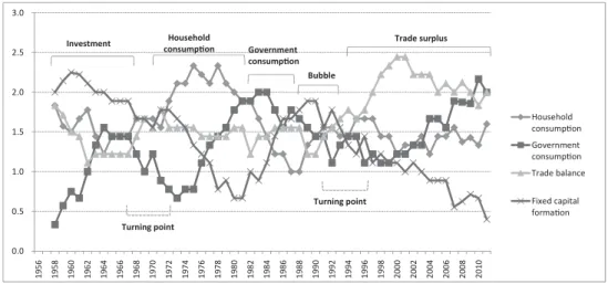
Orbit analysis is a statistical method that extracts leading-following relations between two variables by combining coordinates of time-series data along time and calculating the slope and the direction of rotation of the orbit thus depicted. In the case of many variables, calculations of all combinations between pair variables produce a hierarchy of leading-following relations among all variables (Itaki(2014)), which identifies the kick-starter variable that heralds all variations among other variables and determines their order of following. The method is applied to the four aggregates of Japan s GDP in the same period in Fig. 5 9-year moving average of ranking points for Japan s GDP (expenditure) . Due to wide annual variance of ranking points, 9-year moving average is adopted out of 5-, 7- and 9-year calculations, which seems to represent most appropriately medium-term variations.
Annual changes in value are used for the calculations, because there have to be quantitative pulling- and being-pulled-relations among variables for them to be actually leading-following relations (Itaki (2014) p.16, pp.30-31.). Household consumption, government consumption, trade balance and fixed capital formation are apparently in quantitative pulling- and being-pulled-relations in their annual changes in value. That is not a priori true in their annual growth rates: although an increase in household consumption by 10 billion yen, for example, directly causes quantitative deterioration in trade balance or an increase in fixed capital formation by 1 billion yen or so, its increase by 5 %, for example, does not necessarily cause an increase or decrease in trade balance or fixed capital formation by a certain percentage point. Fig. 5 shows that the kick-starter (i.e. the first leading variable) was fixed capital formation in 1958-67, household consumption in 1972-80, government consumption in the period of fiscal reconstruction 1983-85, fixed capital formation again in the period of an economic bubble and its burst 1988-1992 and trade balance in the period of the great depression 1996-2009. Another feature is that fixed capital formation was in the lowest rank in 1977-84, the period between the aftermath of the first worldwide recession since
Fig. 5: 9-year moving average of ranking points for Japan’s GDP (expenditure)
0.0 0.5 1.0 1.5 2.0 2.5 3.0 Household consumpƟon Government consumpƟon Trade balance Fixed capital formaƟon Investment Household cŽŶƐƵŵƉƟŽŶ Government cŽŶƐƵŵƉƟŽŶ Bubble Trade surplus Turning point Turning point 1956 19 58 19 60 1962 19 64 19 66 1968 19 70 1972 19 74 19 76 1978 1980 1982 1984 19 86 1988 1990 1992 1994 1996 1998 20 00 20 02 2004 20 06 20 08 2010
the end of Second World War, 1974-75, and the previous year of the Plaza Accord in 1985; and that happened again since 2000. Investment in plants and equipments does not now play the role of generating changes in GDP. On top of that, two major structural transformations of Japanese economy took place, first in the end of the 1960s and early 1970s and second in the first half of the 1990s in the aftermath of the burst of bubble, when ranks were intertwined in a bunch and changed quickly. We now know that information acquired by orbit analysis by and large corresponds to our widely shared knowledge about the post-World War history of Japanese economy, and also that it adds many other insights to our understanding.
We ought to pay enough attention to the difference between the two concepts, leading
and following and preceding and lagging 6). The unit of our observation and
analysis is one period of time, the beginning and end of which we can observe and compare, but we do not know actions and reactions that may take place among variables during the minimum one period of time. Therefore, we cannot know, in principle, which variable precedes or lags, or whether reversals in ranks repeat themselves, during the unit period, just like in a black box. What we can actually observe and measure is distinction between a variable that actively leads changes and a variable that follows the changes initiated. Those changes are produced by complicated actions and reactions (positive and negative feedbacks) among variables. The distinction is observed and recorded as if being temporal preceding-lagging relations. We should be careful enough, therefore, that leading-following relations in Fig. 5 among four aggregates are not temporal preceding-lagging relations. Their distinction reveals its importance later when orbit analysis is conducted among the principal components of those four aggregates.
An application of orbit analysis to annual variations in value in Fig. 1 exposes hidden leading-following relations among the aggregates in Fig. 5. It is certainly a big step forwards to the understanding of structure and movements of the object, which, however, touches only its surface; we next proceed to principal component analysis and further to developmental principal component analysis that allow us to investigate more essential and autonomous substance, forces or motive power of the object that is hidden under the surface of those leading-following aggregates.
(3) Principal component analysis 1. Terms
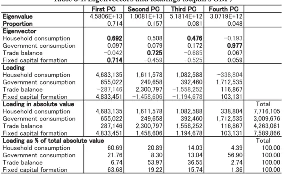
The results of principal component analysis on the four aggregates of Japan s GDP are shown in Table 3-1 Eigenvectors and loadings (Japan s GDP) and Table 4 Principal component scores of Japan s GDP . Explanation of terms in these tables and some features of principal component analysis are given as follows:
Principal component analysis on the basis of variance and of correlation:
there are two types of principal component analysis, one that is based on original data, i.e. their variance, and another on their correlation. The latter is conducted on standardized scores (i.e. Z scores) whose standard deviation is one. Here we adopt the former because the four aggregates share the same monetary unit, i.e. the Japanese
yen, and we would like to conduct orbit analysis and principal component analysis on the basis of monetary value. The latter is usually used in the case in which variables have different units of measurement or in which, despite sharing the same unit, difference in value does not make sense for one reason or another.
Principal components: four principal components are extracted from four
variables. With the first principal component being Z1, household consumption X1, the
government consumption X2, trade balance X3 and fixed capital formation X4, we get Z1
= 0.692 X1 + 0.097 X2− 0.042 X3 + 0.714 X4 from the eigenvector in the table: the first
principal component is composed as a synthetic function of the original four variables. So are the other principal components.
Eigenvector: eigenvectors that consist of the coefficients of the principal components have a property that the sum of squares of all elements in each row and
each column is one: for example, regarding household consumption 0.6922 + 0.5082 +
0.4762 + (−0.193) 2 = 1, and regarding the first principal component 0.6922 + 0.0972 +
(−0.042) 2+ 0.7142 = 1. Values and signs of elements give us an important clue when
we attempt to interpret the meanings of principal components.
Loading: the sum of squares of all loadings of the first principal component, i.e. household consumption 4,683,135, government consumption 65,502, trade balance
㻲㼕㼞㼟㼠 㻼㻯 㻿㼑㼏㼛㼚㼐 㻼㻯 㼀㼔㼕㼞㼐 㻼㻯 㻲㼛㼡㼞㼠㼔 㻼㻯 㻱㼕㼓㼑㼚㼢㼍㼘㼡㼑 㻠㻚㻡㻤㻜㻢㻱㻗㻝㻟 㻝㻚㻜㻜㻤㻝㻱㻗㻝㻟 㻡㻚㻝㻤㻝㻠㻱㻗㻝㻞 㻟㻚㻜㻣㻝㻥㻱㻗㻝㻞 㻼㼞㼛㼜㼛㼞㼠㼕㼛㼚 㻜㻚㻣㻝㻠 㻜㻚㻝㻡㻣 㻜㻚㻜㻤㻝 㻜㻚㻜㻠㻤 㻱㼕㼓㼑㼚㼢㼑㼏㼠㼛㼞 㻴㼛㼡㼟㼑㼔㼛㼘㼐㻌㼏㼛㼚㼟㼡㼙㼜㼠㼕㼛㼚 㻜㻚㻢㻥㻞 㻜㻚㻡㻜㻤 㻜㻚㻠㻣㻢 㻙㻜㻚㻝㻥㻟 㻳㼛㼢㼑㼞㼚㼙㼑㼚㼠㻌㼏㼛㼚㼟㼡㼙㼜㼠㼕㼛㼚 㻜㻚㻜㻥㻣 㻜㻚㻜㻣㻥 㻜㻚㻝㻣㻞 㻜㻚㻥㻣㻣 㼀㼞㼍㼐㼑㻌㼎㼍㼘㼍㼚㼏㼑 㻙㻜㻚㻜㻠㻞 㻜㻚㻣㻞㻡 㻙㻜㻚㻢㻤㻡 㻜㻚㻜㻢㻣 㻲㼕㼤㼑㼐㻌㼏㼍㼜㼕㼠㼍㼘㻌㼒㼛㼞㼙㼍㼠㼕㼛㼚 㻜㻚㻣㻝㻠 㻙㻜㻚㻠㻡㻥 㻙㻜㻚㻡㻞㻡 㻜㻚㻜㻡㻥 㻸㼛㼍㼐㼕㼚㼓 㻴㼛㼡㼟㼑㼔㼛㼘㼐㻌㼏㼛㼚㼟㼡㼙㼜㼠㼕㼛㼚 㻠㻘㻢㻤㻟㻘㻝㻟㻡 㻝㻘㻢㻝㻝㻘㻡㻣㻤 㻝㻘㻜㻤㻞㻘㻡㻤㻤 㻙㻟㻟㻤㻘㻤㻜㻠 㻳㼛㼢㼑㼞㼚㼙㼑㼚㼠㻌㼏㼛㼚㼟㼡㼙㼜㼠㼕㼛㼚 㻢㻡㻡㻘㻜㻞㻞 㻞㻠㻥㻘㻢㻡㻤 㻟㻥㻞㻘㻠㻢㻜 㻝㻘㻣㻝㻞㻘㻡㻟㻡 㼀㼞㼍㼐㼑㻌㼎㼍㼘㼍㼚㼏㼑 㻙㻞㻤㻣㻘㻝㻠㻢 㻞㻘㻟㻜㻜㻘㻣㻥㻣 㻙㻝㻘㻡㻡㻤㻘㻞㻡㻞 㻝㻝㻢㻘㻤㻢㻣 㻲㼕㼤㼑㼐㻌㼏㼍㼜㼕㼠㼍㼘㻌㼒㼛㼞㼙㼍㼠㼕㼛㼚 㻠㻘㻤㻟㻟㻘㻠㻡㻝 㻙㻝㻘㻠㻡㻤㻘㻢㻜㻢 㻙㻝㻘㻝㻥㻠㻘㻢㻣㻤 㻝㻜㻟㻘㻝㻟㻝 㻸㼛㼍㼐㼕㼚㼓 㼕㼚 㼍㼎㼟㼛㼘㼡㼠㼑 㼢㼍㼘㼡㼑 㼀㼛㼠㼍㼘 㻴㼛㼡㼟㼑㼔㼛㼘㼐㻌㼏㼛㼚㼟㼡㼙㼜㼠㼕㼛㼚 㻠㻘㻢㻤㻟㻘㻝㻟㻡 㻝㻘㻢㻝㻝㻘㻡㻣㻤 㻝㻘㻜㻤㻞㻘㻡㻤㻤 㻟㻟㻤㻘㻤㻜㻠 㻣㻘㻣㻝㻢㻘㻝㻜㻡 㻳㼛㼢㼑㼞㼚㼙㼑㼚㼠㻌㼏㼛㼚㼟㼡㼙㼜㼠㼕㼛㼚 㻢㻡㻡㻘㻜㻞㻞 㻞㻠㻥㻘㻢㻡㻤 㻟㻥㻞㻘㻠㻢㻜 㻝㻘㻣㻝㻞㻘㻡㻟㻡 㻟㻘㻜㻜㻥㻘㻢㻣㻢 㼀㼞㼍㼐㼑㻌㼎㼍㼘㼍㼚㼏㼑 㻞㻤㻣㻘㻝㻠㻢 㻞㻘㻟㻜㻜㻘㻣㻥㻣 㻝㻘㻡㻡㻤㻘㻞㻡㻞 㻝㻝㻢㻘㻤㻢㻣 㻠㻘㻞㻢㻟㻘㻜㻢㻝 㻲㼕㼤㼑㼐㻌㼏㼍㼜㼕㼠㼍㼘㻌㼒㼛㼞㼙㼍㼠㼕㼛㼚 㻠㻘㻤㻟㻟㻘㻠㻡㻝 㻝㻘㻠㻡㻤㻘㻢㻜㻢 㻝㻘㻝㻥㻠㻘㻢㻣㻤 㻝㻜㻟㻘㻝㻟㻝 㻣㻘㻡㻤㻥㻘㻤㻢㻢 㻸㼛㼍㼐㼕㼚㼓 㼍㼟 㻑 㼛㼒 㼠㼛㼠㼍㼘 㼍㼎㼟㼛㼘㼡㼠㼑 㼢㼍㼘㼡㼑 㼀㼛㼠㼍㼘 㻴㼛㼡㼟㼑㼔㼛㼘㼐㻌㼏㼛㼚㼟㼡㼙㼜㼠㼕㼛㼚 㻢㻜㻚㻢㻥 㻞㻜㻚㻤㻥 㻝㻠㻚㻜㻟 㻠㻚㻟㻥 㻝㻜㻜㻚㻜㻜 㻳㼛㼢㼑㼞㼚㼙㼑㼚㼠㻌㼏㼛㼚㼟㼡㼙㼜㼠㼕㼛㼚 㻞㻝㻚㻣㻢 㻤㻚㻟㻜 㻝㻟㻚㻜㻠 㻡㻢㻚㻥㻜 㻝㻜㻜㻚㻜㻜 㼀㼞㼍㼐㼑㻌㼎㼍㼘㼍㼚㼏㼑 㻢㻚㻣㻠 㻡㻟㻚㻥㻣 㻟㻢㻚㻡㻡 㻞㻚㻣㻠 㻝㻜㻜㻚㻜㻜 㻲㼕㼤㼑㼐㻌㼏㼍㼜㼕㼠㼍㼘㻌㼒㼛㼞㼙㼍㼠㼕㼛㼚 㻢㻟㻚㻢㻤 㻝㻥㻚㻞㻞 㻝㻡㻚㻣㻠 㻝㻚㻟㻢 㻝㻜㻜㻚㻜㻜
Table 3-1: Eigenvectors and loadings (Japan's GDP)
㻿㼝㼡㼍㼞㼑 㼛㼒 㼘㼛㼍㼐㼕㼚㼓 㻲㼕㼞㼟㼠 㻼㻯 㻿㼑㼏㼛㼚㼐 㻼㻯 㼀㼔㼕㼞㼐 㻼㻯 㻲㼛㼡㼞㼠㼔 㻼㻯 㼀㼛㼠㼍㼘 㼙 㼡 㼟 㼚 㼛 㼏 㼐 㼘 㼛 㼔 㼑 㼟 㼡 㼛 㻴 㼜㼠㼕㼛㼚 㻞㻝㻘㻥㻟㻝㻘㻣㻡㻟㻘㻢㻢㻝㻘㻝㻞㻜 㻞㻘㻡㻥㻣㻘㻝㻤㻞㻘㻜㻢㻡㻘㻜㻣㻢 㻝㻘㻝㻣㻝㻘㻥㻥㻡㻘㻤㻠㻞㻘㻣㻡㻡 㻝㻝㻠㻘㻣㻤㻤㻘㻠㻞㻟㻘㻣㻣㻥 㻞㻡㻘㻤㻝㻡㻘㻣㻝㻥㻘㻥㻥㻞㻘㻣㻟㻜 㼙 㼡 㼟 㼚 㼛 㼏 㼠 㼚 㼑 㼙 㼚 㼞 㼑 㼢 㼛 㻳 㼜㼠㼕㼛㼚 㻠㻞㻥㻘㻜㻡㻟㻘㻢㻤㻞㻘㻜㻞㻟 㻢㻞㻘㻟㻞㻥㻘㻞㻟㻣㻘㻟㻥㻟 㻝㻡㻠㻘㻜㻞㻡㻘㻜㻜㻠㻘㻣㻝㻟 㻞㻘㻥㻟㻞㻘㻣㻣㻣㻘㻟㻠㻢㻘㻜㻡㻟 㻟㻘㻡㻣㻤㻘㻝㻤㻡㻘㻞㻣㻜㻘㻝㻤㻞 㼀㼞㼍㼐㼑㻌㼎㼍㼘㼍㼚㼏㼑 㻤㻞㻘㻠㻡㻞㻘㻣㻤㻡㻘㻞㻤㻡 㻡㻘㻞㻥㻟㻘㻢㻢㻡㻘㻜㻜㻤㻘㻝㻥㻥 㻞㻘㻠㻞㻤㻘㻝㻠㻤㻘㻝㻝㻣㻘㻝㻟㻠 㻝㻟㻘㻢㻡㻣㻘㻥㻢㻢㻘㻠㻤㻥 㻣㻘㻤㻝㻣㻘㻥㻞㻟㻘㻤㻣㻣㻘㻝㻜㻣 㻲㼕㼤㼑㼐㻌㼏㼍㼜㼕㼠㼍㼘㻌㼒㼛㼞㼙㼍㼠㼕㼛㼚 㻞㻟㻘㻟㻢㻞㻘㻞㻡㻜㻘㻝㻥㻞㻘㻢㻠㻠 㻞㻘㻝㻞㻣㻘㻡㻟㻞㻘㻟㻞㻤㻘㻝㻝㻥 㻝㻘㻠㻞㻣㻘㻞㻡㻢㻘㻟㻞㻞㻘㻟㻠㻝 㻝㻜㻘㻢㻟㻡㻘㻥㻝㻠㻘㻥㻢㻠 㻞㻢㻘㻥㻞㻣㻘㻢㻣㻠㻘㻣㻡㻤㻘㻜㻢㻣 㼀㼛㼠㼍㼘 㻠㻡㻘㻤㻜㻡㻘㻡㻝㻜㻘㻟㻞㻝㻘㻜㻣㻞 㻝㻜㻘㻜㻤㻜㻘㻣㻜㻤㻘㻢㻟㻤㻘㻣㻤㻢 㻡㻘㻝㻤㻝㻘㻠㻞㻡㻘㻞㻤㻢㻘㻥㻠㻟 㻟㻘㻜㻣㻝㻘㻤㻡㻥㻘㻢㻡㻝㻘㻞㻤㻡 㻢㻠㻘㻝㻟㻥㻘㻡㻜㻟㻘㻤㻥㻤㻘㻜㻤㻢
−287,146 and fixed capital formation 4,833,451 is equal to the eigenvalue 45,805,510,321,072. This holds true for the second principal component and others. Loadings represent composition of an eigenvalue of each principal component and give us another important clue, in addition to eigenvectors, when we attempt to interpret the meanings of principal components.
Eigenvalue and its proportion: the sum of eigenvalues of all principal components is equal to the variance of the original variables, which is shown in Table 3-2 Square of loadings (Japan s GDP) : all information about the variance of the original variables is turned into that of the principal components. As in Table 3-1, the
㻲㼕㼞㼟㼠㻌㻼㻯 㻿㼑㼏㼛㼚㼐㻌㻼㻯 㼀㼔㼕㼞㼐㻌㻼㻯 㻲㼛㼡㼞㼠㼔㻌㻼㻯 㻲㼕㼞㼟㼠㻌㻼㻯 㻿㼑㼏㼛㼚㼐㻌㻼㻯 㼀㼔㼕㼞㼐㻌㻼㻯 㻲㼛㼡㼞㼠㼔㻌㻼㻯 㻝㻥㻡㻢 㻙㻠㻘㻜㻥㻣㻘㻝㻤㻡 㻙㻝㻘㻣㻢㻟㻘㻝㻟㻣 㻙㻝㻘㻤㻜㻥㻘㻣㻢㻢 㻙㻤㻠㻝㻘㻢㻠㻤 㻣㻢㻤㻘㻝㻤㻞 㻙㻝㻤㻘㻤㻥㻤 㻡㻢㻘㻞㻤㻡 㻙㻡㻡㻘㻞㻟㻜 㻝㻥㻡㻣 㻙㻟㻘㻤㻤㻡㻘㻞㻥㻜 㻙㻝㻘㻣㻥㻥㻘㻢㻣㻡 㻙㻝㻘㻣㻞㻞㻘㻤㻜㻠 㻙㻤㻟㻞㻘㻢㻣㻝 㻥㻤㻜㻘㻜㻣㻣 㻙㻡㻡㻘㻠㻟㻢 㻝㻠㻟㻘㻞㻠㻤 㻙㻠㻢㻘㻞㻡㻞 㻝㻥㻡㻤 㻙㻠㻘㻠㻤㻡㻘㻤㻟㻝 㻙㻝㻘㻞㻠㻝㻘㻠㻠㻟 㻙㻝㻘㻥㻞㻞㻘㻡㻟㻟 㻙㻣㻣㻠㻘㻢㻤㻜 㻟㻣㻥㻘㻡㻟㻢 㻡㻜㻞㻘㻣㻥㻢 㻙㻡㻢㻘㻠㻤㻝 㻝㻝㻘㻣㻟㻥 㻝㻥㻡㻥 㻙㻟㻘㻤㻤㻤㻘㻝㻠㻟 㻙㻝㻘㻡㻟㻥㻘㻢㻤㻡 㻙㻝㻘㻢㻤㻤㻘㻠㻞㻞 㻙㻤㻟㻟㻘㻥㻥㻢 㻥㻣㻣㻘㻞㻞㻠 㻞㻜㻠㻘㻡㻡㻠 㻝㻣㻣㻘㻢㻞㻥 㻙㻠㻣㻘㻡㻣㻤 㻝㻥㻢㻜 㻙㻟㻘㻜㻤㻠㻘㻝㻠㻜 㻙㻝㻘㻣㻟㻜㻘㻡㻡㻜 㻙㻝㻘㻤㻡㻥㻘㻟㻢㻡 㻙㻣㻥㻢㻘㻠㻢㻥 㻝㻘㻣㻤㻝㻘㻞㻞㻣 㻝㻟㻘㻢㻤㻥 㻢㻘㻢㻤㻣 㻙㻝㻜㻘㻜㻡㻝 㻝㻥㻢㻝 㻙㻞㻘㻢㻜㻡㻘㻤㻤㻞 㻙㻝㻘㻤㻣㻢㻘㻣㻟㻞 㻙㻝㻘㻡㻥㻡㻘㻜㻝㻠 㻙㻤㻠㻜㻘㻝㻠㻜 㻞㻘㻞㻡㻥㻘㻠㻤㻡 㻙㻝㻟㻞㻘㻠㻥㻟 㻞㻣㻝㻘㻜㻟㻤 㻙㻡㻟㻘㻣㻞㻝 㻝㻥㻢㻞 㻙㻟㻘㻜㻥㻜㻘㻠㻢㻤 㻙㻝㻘㻜㻢㻟㻘㻟㻡㻠 㻙㻝㻘㻣㻡㻡㻘㻥㻤㻢 㻙㻣㻢㻣㻘㻣㻤㻣 㻝㻘㻣㻣㻠㻘㻤㻥㻥 㻢㻤㻜㻘㻤㻤㻡 㻝㻝㻜㻘㻜㻢㻢 㻝㻤㻘㻢㻟㻝 㻝㻥㻢㻟 㻙㻞㻘㻣㻠㻜㻘㻠㻠㻢 㻙㻝㻘㻞㻝㻠㻘㻣㻤㻜 㻙㻝㻘㻜㻥㻝㻘㻞㻤㻜 㻙㻤㻠㻡㻘㻡㻠㻝 㻞㻘㻝㻞㻠㻘㻥㻞㻝 㻡㻞㻥㻘㻠㻡㻥 㻣㻣㻠㻘㻣㻣㻞 㻙㻡㻥㻘㻝㻞㻟 㻝㻥㻢㻠 㻙㻞㻘㻞㻢㻜㻘㻟㻢㻠 㻙㻝㻘㻝㻞㻠㻘㻜㻢㻠 㻙㻝㻘㻢㻜㻝㻘㻥㻡㻤 㻙㻤㻡㻞㻘㻠㻠㻤 㻞㻘㻢㻜㻡㻘㻜㻜㻟 㻢㻞㻜㻘㻝㻣㻡 㻞㻢㻠㻘㻜㻥㻠 㻙㻢㻢㻘㻜㻟㻜 㻝㻥㻢㻡 㻙㻟㻘㻜㻞㻠㻘㻝㻣㻤 㻙㻠㻝㻣㻘㻤㻞㻝 㻙㻝㻘㻟㻞㻢㻘㻤㻜㻤 㻙㻤㻞㻠㻘㻠㻡㻢 㻝㻘㻤㻠㻝㻘㻝㻤㻥 㻝㻘㻟㻞㻢㻘㻠㻝㻤 㻡㻟㻥㻘㻞㻠㻟 㻙㻟㻤㻘㻜㻟㻤 㻝㻥㻢㻢 㻙㻝㻘㻡㻡㻢㻘㻡㻠㻝 㻙㻥㻢㻜㻘㻝㻞㻢 㻙㻝㻘㻠㻡㻜㻘㻠㻜㻞 㻙㻤㻣㻣㻘㻣㻢㻣 㻟㻘㻟㻜㻤㻘㻤㻞㻢 㻣㻤㻠㻘㻝㻝㻟 㻠㻝㻡㻘㻢㻡㻜 㻙㻥㻝㻘㻟㻠㻥 㻝㻥㻢㻣 㻙㻢㻜㻡㻘㻞㻡㻤 㻙㻝㻘㻢㻣㻞㻘㻞㻟㻢 㻙㻝㻘㻟㻠㻟㻘㻠㻡㻣 㻙㻥㻠㻞㻘㻝㻡㻟 㻠㻘㻞㻢㻜㻘㻝㻜㻥 㻣㻞㻘㻜㻜㻟 㻡㻞㻞㻘㻡㻥㻡 㻙㻝㻡㻡㻘㻣㻟㻡 㻝㻥㻢㻤 㻙㻞㻠㻘㻝㻜㻞 㻙㻝㻘㻜㻠㻟㻘㻝㻤㻡 㻙㻞㻘㻝㻟㻡㻘㻞㻡㻢 㻙㻣㻟㻤㻘㻡㻤㻠 㻠㻘㻤㻠㻝㻘㻞㻢㻡 㻣㻜㻝㻘㻜㻡㻠 㻙㻞㻢㻥㻘㻞㻜㻡 㻠㻣㻘㻤㻟㻡 㻝㻥㻢㻥 㻥㻟㻣㻘㻥㻠㻟 㻙㻥㻤㻣㻘㻥㻥㻞 㻙㻞㻘㻜㻜㻤㻘㻢㻟㻥 㻙㻣㻡㻤㻘㻝㻝㻜 㻡㻘㻤㻜㻟㻘㻟㻝㻜 㻣㻡㻢㻘㻞㻠㻣 㻙㻝㻠㻞㻘㻡㻤㻤 㻞㻤㻘㻟㻜㻤 㻝㻥㻣㻜 㻝㻘㻥㻥㻟㻘㻜㻜㻡 㻙㻝㻘㻞㻣㻜㻘㻟㻥㻝 㻙㻝㻘㻢㻥㻤㻘㻣㻥㻥 㻙㻢㻝㻡㻘㻠㻣㻜 㻢㻘㻤㻡㻤㻘㻟㻣㻞 㻠㻣㻟㻘㻤㻠㻤 㻝㻢㻣㻘㻞㻡㻟 㻝㻣㻜㻘㻥㻠㻤 㻝㻥㻣㻝 㻙㻞㻥㻣㻘㻥㻢㻣 㻥㻥㻢㻘㻟㻢㻤 㻙㻝㻘㻜㻢㻣㻘㻠㻡㻥 㻙㻢㻝㻝㻘㻠㻠㻠 㻠㻘㻡㻢㻣㻘㻠㻜㻜 㻞㻘㻣㻠㻜㻘㻢㻜㻣 㻣㻥㻤㻘㻡㻥㻟 㻝㻣㻠㻘㻥㻣㻠 㻝㻥㻣㻞 㻞㻘㻢㻟㻢㻘㻤㻠㻝 㻙㻝㻜㻞㻘㻝㻠㻝 㻙㻠㻥㻣㻘㻞㻤㻡 㻙㻣㻢㻝㻘㻣㻡㻝 㻣㻘㻡㻜㻞㻘㻞㻜㻤 㻝㻘㻢㻠㻞㻘㻜㻥㻤 㻝㻘㻟㻢㻤㻘㻣㻢㻢 㻞㻠㻘㻢㻢㻣 㻝㻥㻣㻟 㻥㻘㻟㻞㻞㻘㻤㻞㻤 㻙㻞㻘㻝㻣㻜㻘㻞㻢㻠 㻙㻝㻜㻣㻘㻝㻝㻝 㻙㻢㻞㻢㻘㻜㻤㻝 㻝㻠㻘㻝㻤㻤㻘㻝㻥㻡 㻙㻠㻞㻢㻘㻜㻞㻡 㻝㻘㻣㻡㻤㻘㻥㻠㻜 㻝㻢㻜㻘㻟㻟㻣 㻝㻥㻣㻠 㻤㻘㻞㻥㻝㻘㻥㻝㻢 㻝㻘㻠㻥㻝㻘㻞㻞㻠 㻞㻘㻟㻝㻞㻘㻣㻜㻞 㻙㻝㻝㻡㻘㻠㻟㻞 㻝㻟㻘㻝㻡㻣㻘㻞㻤㻟 㻟㻘㻞㻟㻡㻘㻠㻢㻟 㻠㻘㻝㻣㻤㻘㻣㻡㻟 㻢㻣㻜㻘㻥㻤㻢 㻝㻥㻣㻡 㻠㻘㻡㻣㻡㻘㻞㻠㻟 㻠㻘㻡㻤㻢㻘㻣㻠㻜 㻞㻘㻣㻠㻟㻘㻥㻟㻠 㻙㻟㻟㻞㻘㻠㻡㻜 㻥㻘㻠㻠㻜㻘㻢㻝㻜 㻢㻘㻟㻟㻜㻘㻥㻣㻥 㻠㻘㻢㻜㻥㻘㻥㻤㻢 㻠㻡㻟㻘㻥㻢㻤 㻝㻥㻣㻢 㻡㻘㻡㻣㻡㻘㻜㻢㻣 㻟㻘㻝㻠㻞㻘㻝㻢㻠 㻣㻢㻤㻘㻞㻡㻞 㻙㻝㻘㻝㻝㻡㻘㻤㻟㻝 㻝㻜㻘㻠㻠㻜㻘㻠㻟㻠 㻠㻘㻤㻤㻢㻘㻠㻜㻟 㻞㻘㻢㻟㻠㻘㻟㻜㻠 㻙㻟㻞㻥㻘㻠㻝㻟 㻝㻥㻣㻣 㻡㻘㻥㻟㻡㻘㻣㻤㻠 㻟㻘㻡㻝㻞㻘㻟㻞㻤 㻡㻟㻟㻘㻠㻝㻝 㻙㻤㻟㻟㻘㻥㻜㻟 㻝㻜㻘㻤㻜㻝㻘㻝㻡㻝 㻡㻘㻞㻡㻢㻘㻡㻢㻣 㻞㻘㻟㻥㻥㻘㻠㻢㻟 㻙㻠㻣㻘㻠㻤㻡 㻝㻥㻣㻤 㻣㻘㻝㻢㻣㻘㻝㻟㻢 㻝㻘㻠㻞㻜㻘㻢㻥㻣 㻙㻟㻠㻘㻢㻤㻟 㻙㻝㻘㻜㻝㻝㻘㻠㻞㻡 㻝㻞㻘㻜㻟㻞㻘㻡㻜㻟 㻟㻘㻝㻢㻠㻘㻥㻟㻢 㻝㻘㻤㻟㻝㻘㻟㻢㻥 㻙㻞㻞㻡㻘㻜㻜㻣 㻝㻥㻣㻥 㻥㻘㻢㻣㻥㻘㻞㻡㻜 㻙㻟㻘㻝㻡㻜㻘㻣㻣㻟 㻟㻘㻤㻜㻡㻘㻢㻟㻡 㻙㻝㻘㻟㻠㻜㻘㻟㻠㻠 㻝㻠㻘㻡㻠㻠㻘㻢㻝㻣 㻙㻝㻘㻠㻜㻢㻘㻡㻟㻠 㻡㻘㻢㻣㻝㻘㻢㻤㻣 㻙㻡㻡㻟㻘㻥㻞㻢 㻝㻥㻤㻜 㻞㻘㻤㻜㻢㻘㻞㻠㻝 㻙㻞㻘㻥㻡㻤㻘㻥㻞㻟 㻙㻞㻘㻜㻥㻞㻘㻜㻢㻥 㻝㻝㻘㻣㻜㻥㻘㻜㻟㻢 㻣㻘㻢㻣㻝㻘㻢㻜㻤 㻙㻝㻘㻞㻝㻠㻘㻢㻤㻠 㻙㻞㻞㻢㻘㻜㻝㻤 㻝㻞㻘㻠㻥㻡㻘㻠㻡㻠 㻝㻥㻤㻝 㻟㻘㻟㻞㻢㻘㻟㻝㻟 㻠㻘㻞㻤㻢㻘㻞㻤㻜 㻙㻝㻘㻥㻜㻠㻘㻠㻥㻥 㻡㻡㻢㻘㻤㻢㻤 㻤㻘㻝㻥㻝㻘㻢㻤㻜 㻢㻘㻜㻟㻜㻘㻡㻝㻥 㻙㻟㻤㻘㻠㻠㻤 㻝㻘㻟㻠㻟㻘㻞㻤㻢 㻝㻥㻤㻞 㻞㻘㻥㻥㻢㻘㻡㻠㻥 㻟㻘㻞㻥㻡㻘㻤㻞㻥 㻟㻘㻝㻝㻜㻘㻣㻢㻝 㻙㻡㻝㻟㻘㻤㻡㻟 㻣㻘㻤㻢㻝㻘㻥㻝㻢 㻡㻘㻜㻠㻜㻘㻜㻢㻤 㻠㻘㻥㻣㻢㻘㻤㻝㻞 㻞㻣㻞㻘㻡㻢㻡 㻝㻥㻤㻟 㻙㻞㻟㻤㻘㻠㻠㻜 㻡㻘㻟㻝㻣㻘㻟㻝㻟 㻥㻥㻤㻘㻞㻜㻥 㻣㻥㻘㻥㻝㻟 㻠㻘㻢㻞㻢㻘㻥㻞㻣 㻣㻘㻜㻢㻝㻘㻡㻡㻞 㻞㻘㻤㻢㻠㻘㻞㻢㻜 㻤㻢㻢㻘㻟㻟㻞 㻝㻥㻤㻠 㻟㻘㻡㻟㻥㻘㻞㻝㻡 㻟㻘㻝㻝㻝㻘㻡㻤㻤 㻙㻝㻘㻤㻜㻝㻘㻟㻞㻝 㻙㻞㻝㻘㻤㻝㻜 㻤㻘㻠㻜㻠㻘㻡㻤㻞 㻠㻘㻤㻡㻡㻘㻤㻞㻣 㻢㻠㻘㻣㻟㻜 㻣㻢㻠㻘㻢㻜㻤 㻝㻥㻤㻡 㻢㻘㻢㻤㻞㻘㻟㻡㻞 㻞㻘㻞㻥㻞㻘㻜㻝㻝 㻙㻞㻘㻢㻟㻡㻘㻜㻡㻢 㻙㻝㻡㻣㻘㻥㻟㻢 㻝㻝㻘㻡㻠㻣㻘㻣㻝㻥 㻠㻘㻜㻟㻢㻘㻞㻡㻜 㻙㻣㻢㻥㻘㻜㻜㻡 㻢㻞㻤㻘㻠㻤㻟 㻝㻥㻤㻢 㻟㻘㻞㻜㻠㻘㻢㻞㻤 㻝㻘㻤㻥㻤㻘㻝㻥㻟 㻙㻝㻘㻢㻤㻡㻘㻟㻡㻟 㻞㻟㻠㻘㻠㻡㻤 㻤㻘㻜㻢㻥㻘㻥㻥㻡 㻟㻘㻢㻠㻞㻘㻠㻟㻞 㻝㻤㻜㻘㻢㻥㻥 㻝㻘㻜㻞㻜㻘㻤㻣㻣 㻝㻥㻤㻣 㻢㻘㻞㻡㻠㻘㻢㻝㻣 㻙㻞㻘㻟㻟㻢㻘㻡㻤㻤 㻤㻠㻠㻘㻣㻠㻝 㻙㻞㻟㻞㻘㻟㻠㻥 㻝㻝㻘㻝㻝㻥㻘㻥㻤㻠 㻙㻡㻥㻞㻘㻟㻠㻥 㻞㻘㻣㻝㻜㻘㻣㻥㻞 㻡㻡㻠㻘㻜㻢㻥 㻝㻥㻤㻤 㻝㻞㻘㻢㻣㻥㻘㻞㻝㻠 㻙㻠㻘㻜㻤㻡㻘㻡㻞㻥 㻙㻝㻘㻥㻢㻥㻘㻣㻜㻠 㻙㻢㻠㻘㻠㻞㻝 㻝㻣㻘㻡㻠㻠㻘㻡㻤㻝 㻙㻞㻘㻟㻠㻝㻘㻞㻥㻜 㻙㻝㻜㻟㻘㻢㻡㻟 㻣㻞㻝㻘㻥㻥㻣 㻝㻥㻤㻥 㻝㻡㻘㻜㻣㻞㻘㻣㻜㻞 㻙㻞㻘㻜㻜㻟㻘㻟㻜㻢 㻙㻟㻟㻡㻘㻝㻥㻥 㻠㻜㻢㻘㻜㻢㻡 㻝㻥㻘㻥㻟㻤㻘㻜㻢㻥 㻙㻞㻡㻥㻘㻜㻢㻣 㻝㻘㻡㻟㻜㻘㻤㻡㻟 㻝㻘㻝㻥㻞㻘㻠㻤㻟 㻝㻥㻥㻜 㻝㻣㻘㻠㻡㻣㻘㻟㻞㻝 㻙㻢㻞㻜㻘㻞㻣㻝 㻝㻘㻜㻣㻣㻘㻜㻤㻠 㻠㻢㻡㻘㻝㻤㻞 㻞㻞㻘㻟㻞㻞㻘㻢㻤㻤 㻝㻘㻝㻞㻟㻘㻥㻢㻤 㻞㻘㻥㻠㻟㻘㻝㻟㻡 㻝㻘㻞㻡㻝㻘㻢㻜㻜 㻝㻥㻥㻝 㻤㻘㻟㻤㻡㻘㻥㻢㻜 㻟㻘㻤㻥㻞㻘㻞㻣㻜 㻙㻝㻘㻠㻞㻡㻘㻜㻠㻜 㻝㻘㻡㻝㻟㻘㻤㻝㻟 㻝㻟㻘㻞㻡㻝㻘㻟㻞㻣 㻡㻘㻢㻟㻢㻘㻡㻜㻥 㻠㻠㻝㻘㻜㻝㻞 㻞㻘㻟㻜㻜㻘㻞㻟㻞 㻝㻥㻥㻞 㻞㻥㻡㻘㻟㻡㻠 㻢㻘㻠㻠㻝㻘㻥㻜㻤 㻞㻘㻠㻣㻟㻘㻡㻝㻟 㻤㻟㻠㻘㻤㻠㻤 㻡㻘㻝㻢㻜㻘㻣㻞㻝 㻤㻘㻝㻤㻢㻘㻝㻠㻣 㻠㻘㻟㻟㻥㻘㻡㻢㻡 㻝㻘㻢㻞㻝㻘㻞㻢㻢 㻝㻥㻥㻟 㻙㻠㻘㻟㻤㻤㻘㻤㻢㻞 㻟㻘㻢㻟㻜㻘㻡㻡㻠 㻟㻘㻟㻥㻤㻘㻡㻞㻝 㻢㻣㻜㻘㻣㻝㻥 㻠㻣㻢㻘㻡㻜㻠 㻡㻘㻟㻣㻠㻘㻣㻥㻟 㻡㻘㻞㻢㻠㻘㻡㻣㻞 㻝㻘㻠㻡㻣㻘㻝㻟㻣 㻝㻥㻥㻠 㻞㻘㻤㻟㻢㻘㻝㻡㻥 㻡㻘㻞㻥㻥㻘㻡㻞㻥 㻢㻘㻡㻜㻤㻘㻜㻞㻞 㻙㻝㻥㻘㻥㻜㻣 㻣㻘㻣㻜㻝㻘㻡㻞㻢 㻣㻘㻜㻠㻟㻘㻣㻢㻤 㻤㻘㻟㻣㻠㻘㻜㻣㻠 㻣㻢㻢㻘㻡㻝㻝 㻝㻥㻥㻡 㻙㻞㻘㻟㻟㻣㻘㻟㻡㻜 㻙㻝㻘㻠㻢㻝㻘㻝㻜㻣 㻞㻘㻥㻣㻟㻘㻜㻠㻤 㻝㻘㻡㻝㻢㻘㻟㻡㻥 㻞㻘㻡㻞㻤㻘㻜㻝㻣 㻞㻤㻟㻘㻝㻟㻞 㻠㻘㻤㻟㻥㻘㻜㻥㻥 㻞㻘㻟㻜㻞㻘㻣㻣㻤 㻝㻥㻥㻢 㻟㻘㻠㻟㻝㻘㻥㻡㻤 㻙㻟㻘㻣㻡㻝㻘㻟㻟㻝 㻞㻘㻝㻞㻡㻘㻟㻡㻝 㻣㻟㻡㻘㻜㻟㻤 㻤㻘㻞㻥㻣㻘㻟㻞㻡 㻙㻞㻘㻜㻜㻣㻘㻜㻥㻟 㻟㻘㻥㻥㻝㻘㻠㻜㻟 㻝㻘㻡㻞㻝㻘㻠㻡㻣 㻝㻥㻥㻣 㻙㻢㻠㻞㻘㻢㻜㻜 㻟㻘㻢㻣㻡㻘㻟㻥㻟 㻙㻝㻘㻜㻥㻝㻘㻝㻟㻣 㻙㻝㻜㻣㻘㻢㻞㻣 㻠㻘㻞㻞㻞㻘㻣㻢㻣 㻡㻘㻠㻝㻥㻘㻢㻟㻞 㻣㻣㻠㻘㻥㻝㻡 㻢㻣㻤㻘㻣㻥㻝 㻝㻥㻥㻤 㻙㻝㻡㻘㻝㻡㻤㻘㻣㻟㻞 㻡㻘㻠㻟㻟㻘㻢㻝㻠 㻣㻝㻞㻘㻝㻣㻥 㻝㻢㻜㻘㻣㻡㻤 㻙㻝㻜㻘㻞㻥㻟㻘㻟㻢㻡 㻣㻘㻝㻣㻣㻘㻤㻡㻟 㻞㻘㻡㻣㻤㻘㻞㻟㻜 㻥㻠㻣㻘㻝㻣㻣 㻝㻥㻥㻥 㻙㻢㻘㻟㻜㻞㻘㻤㻟㻞 㻙㻠㻜㻝㻘㻣㻣㻣 㻝㻘㻥㻣㻠㻘㻝㻡㻝 㻝㻡㻜㻘㻜㻤㻢 㻙㻝㻘㻠㻟㻣㻘㻠㻢㻡 㻝㻘㻟㻠㻞㻘㻠㻢㻞 㻟㻘㻤㻠㻜㻘㻞㻜㻟 㻥㻟㻢㻘㻡㻜㻡 㻞㻜㻜㻜 㻙㻡㻘㻝㻟㻤㻘㻤㻟㻞 㻙㻞㻘㻞㻠㻡㻘㻝㻢㻝 㻙㻝㻘㻝㻞㻤㻘㻠㻥㻥 㻞㻘㻠㻜㻢㻘㻟㻤㻥 㻙㻞㻣㻟㻘㻠㻢㻡 㻙㻡㻜㻜㻘㻥㻞㻞 㻣㻟㻣㻘㻡㻡㻞 㻟㻘㻝㻥㻞㻘㻤㻜㻤 㻞㻜㻜㻝 㻙㻣㻘㻞㻥㻥㻘㻤㻢㻢 㻙㻝㻘㻜㻡㻤㻘㻞㻟㻞 㻡㻘㻟㻜㻠㻘㻥㻥㻞 㻝㻘㻡㻡㻥㻘㻟㻥㻞 㻙㻞㻘㻠㻟㻠㻘㻠㻥㻥 㻢㻤㻢㻘㻜㻜㻣 㻣㻘㻝㻣㻝㻘㻜㻠㻠 㻞㻘㻟㻠㻡㻘㻤㻝㻝 㻞㻜㻜㻞 㻙㻝㻝㻘㻡㻟㻜㻘㻠㻢㻠 㻠㻘㻠㻣㻢㻘㻤㻝㻜 㻞㻝㻣㻘㻥㻡㻝 㻢㻥㻡㻘㻢㻜㻝 㻙㻢㻘㻢㻢㻡㻘㻜㻥㻣 㻢㻘㻞㻞㻝㻘㻜㻠㻤 㻞㻘㻜㻤㻠㻘㻜㻜㻟 㻝㻘㻠㻤㻞㻘㻜㻝㻥 㻞㻜㻜㻟 㻙㻣㻘㻠㻜㻞㻘㻜㻤㻥 㻙㻠㻣㻝㻘㻠㻟㻤 㻙㻞㻘㻢㻜㻥㻘㻜㻟㻠 㻙㻠㻢㻤㻘㻟㻜㻢 㻙㻞㻘㻡㻟㻢㻘㻣㻞㻞 㻝㻘㻞㻣㻞㻘㻤㻜㻝 㻙㻣㻠㻞㻘㻥㻤㻞 㻟㻝㻤㻘㻝㻝㻞 㻞㻜㻜㻠 㻙㻠㻘㻠㻟㻥㻘㻣㻢㻣 㻞㻝㻞㻘㻤㻡㻥 㻙㻞㻘㻝㻞㻜㻘㻜㻜㻞 㻙㻟㻢㻞㻘㻞㻜㻝 㻠㻞㻡㻘㻢㻜㻜 㻝㻘㻥㻡㻣㻘㻜㻥㻤 㻙㻞㻡㻟㻘㻥㻡㻝 㻠㻞㻠㻘㻞㻝㻤 㻞㻜㻜㻡 㻙㻞㻘㻟㻣㻤㻘㻥㻡㻟 㻙㻞㻘㻣㻤㻜㻘㻞㻠㻞 㻥㻝㻡㻘㻠㻡㻞 㻙㻤㻢㻤㻘㻝㻟㻢 㻞㻘㻠㻤㻢㻘㻠㻝㻠 㻙㻝㻘㻜㻟㻢㻘㻜㻜㻟 㻞㻘㻣㻤㻝㻘㻡㻜㻠 㻙㻤㻝㻘㻣㻝㻤 㻞㻜㻜㻢 㻙㻝㻘㻢㻟㻞㻘㻤㻜㻝 㻙㻞㻘㻞㻜㻤㻘㻣㻝㻣 㻙㻝㻘㻡㻤㻜㻘㻝㻤㻣 㻙㻝㻘㻢㻟㻟㻘㻟㻟㻟 㻟㻘㻞㻟㻞㻘㻡㻢㻢 㻙㻠㻢㻠㻘㻠㻣㻤 㻞㻤㻡㻘㻤㻢㻠 㻙㻤㻠㻢㻘㻥㻝㻠 㻞㻜㻜㻣 㻙㻟㻘㻣㻣㻠㻘㻠㻠㻡 㻙㻢㻡㻘㻢㻞㻣 㻙㻟㻘㻠㻟㻤㻘㻤㻞㻜 㻥㻠㻘㻜㻟㻢 㻝㻘㻜㻥㻜㻘㻥㻞㻞 㻝㻘㻢㻣㻤㻘㻢㻝㻞 㻙㻝㻘㻡㻣㻞㻘㻣㻢㻥 㻤㻤㻜㻘㻠㻡㻠 㻞㻜㻜㻤 㻙㻤㻘㻟㻝㻣㻘㻜㻟㻜 㻙㻢㻘㻤㻟㻝㻘㻜㻤㻠 㻠㻘㻞㻜㻟㻘㻣㻡㻞 㻙㻤㻣㻠㻘㻟㻥㻤 㻙㻟㻘㻠㻡㻝㻘㻢㻢㻟 㻙㻡㻘㻜㻤㻢㻘㻤㻠㻡 㻢㻘㻜㻢㻥㻘㻤㻜㻟 㻙㻤㻣㻘㻥㻤㻜 㻞㻜㻜㻥 㻙㻞㻝㻘㻠㻢㻝㻘㻟㻣㻠 㻤㻤㻣㻘㻢㻣㻜 㻝㻘㻜㻝㻢㻘㻠㻞㻠 㻥㻡㻡㻘㻥㻡㻢 㻙㻝㻢㻘㻡㻥㻢㻘㻜㻜㻣 㻞㻘㻢㻟㻝㻘㻥㻜㻥 㻞㻘㻤㻤㻞㻘㻠㻣㻢 㻝㻘㻣㻠㻞㻘㻟㻣㻠 㻞㻜㻝㻜 㻙㻟㻘㻥㻥㻥㻘㻠㻟㻡 㻟㻘㻠㻤㻡㻘㻝㻡㻤 㻙㻞㻘㻝㻥㻟㻘㻤㻣㻜 㻝㻜㻠㻘㻠㻥㻤 㻤㻢㻡㻘㻥㻟㻞 㻡㻘㻞㻞㻥㻘㻟㻥㻣 㻙㻟㻞㻣㻘㻤㻝㻥 㻤㻥㻜㻘㻥㻝㻣 㻞㻜㻝㻝 㻙㻠㻘㻣㻢㻥㻘㻞㻢㻝 㻙㻥㻘㻢㻥㻞㻘㻠㻠㻡 㻠㻘㻠㻡㻜㻘㻞㻥㻤 㻙㻝㻣㻜㻘㻥㻢㻠 㻥㻢㻘㻝㻜㻢 㻙㻣㻘㻥㻠㻤㻘㻞㻜㻢 㻢㻘㻟㻝㻢㻘㻟㻡㻜 㻢㻝㻡㻘㻠㻡㻠 㻞㻜㻝㻞 㻝㻘㻣㻣㻡㻘㻟㻟㻝 㻙㻠㻘㻢㻤㻢㻘㻟㻣㻞 㻞㻘㻞㻡㻤㻘㻠㻟㻢 㻙㻠㻢㻟㻘㻝㻥㻜 㻢㻘㻢㻠㻜㻘㻢㻥㻤 㻙㻞㻘㻥㻠㻞㻘㻝㻟㻟 㻠㻘㻝㻞㻠㻘㻠㻤㻣 㻟㻞㻟㻘㻞㻞㻤 㻼㼞㼕㼚㼏㼕㼜㼍㼘 㼏㼛㼙㼜㼛㼚㼑㼚㼠 㼟㼏㼛㼞㼑㼟 䠄㼙㼑㼍㼚䠙㻜䠅 㻼㼞㼕㼚㼏㼕㼜㼍㼘 㼏㼛㼙㼜㼛㼚㼑㼚㼠 㼟㼏㼛㼞㼑㼟 䠄㼙㼑㼍㼚䍴㻜䠅 Table 4: Principal component scores of Japan's GDP (unit: 1 million yen)
eigenvalue of the first principal component is the largest and that of the fourth principal component is the smallest. The share of the eigenvalue of each principal component in the total eigenvalue is shown as its proportion: the first principal component contains 71.4% of variance of those four variables, the second 15.7%, the third 8.1% and the fourth 4.8% in the decreasing order. Therefore, the first and second principal components with 87.1% in total can explain most of the variance of all the variables. Principal component analysis has the function of effectively summarizing the number of variables.
Generally speaking, the higher the correlations among the original variables are, the larger the proportion of the first principal component is and the more quickly the proportions of the second and other principal components decrease. To the contrary, when the correlations are low, the proportion of the first principal component becomes small and those of the second and others decrease slowly. Principal component analysis on the basis of correlation of variables with no correlations with each other will produce the same proportions among principal components: for example, 0.2 each for five principal components.
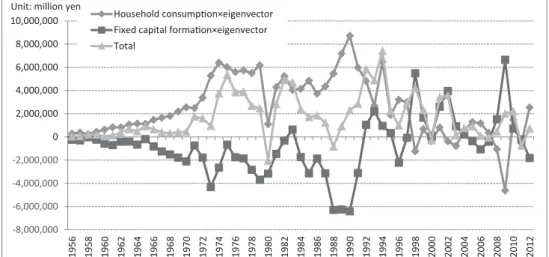
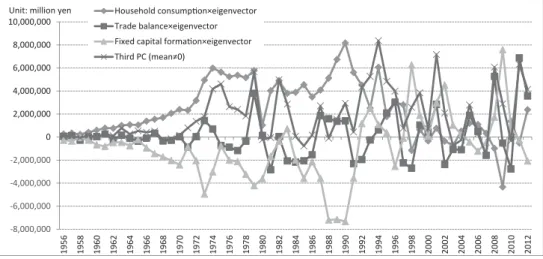
Principal component scores: they are time-series values of each principal
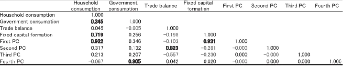
component that are calculated by means of coefficients in an eigenvector (see Table 4 Principal component scores of Japan s GDP ). They are usually calculated with their mean being zero; scores with their mean not being zero are also calculated in the table. Correlations among variables and principal components: Table 5 Correlation matrix (Japan s GDP) provides correlation coefficients between variables, between variables and principal components and between principal components. As stated above, all principal components are orthogonal to each other and thus, their correlation coefficients are all zero. By contrast, in the case of principal component analysis on the basis of correlation, the order of correlation coefficients between variables and principal components is the same as that of coefficients in an eigenvector, and their correlation coefficients are the same as the loadings. In the case of principal component analysis on the basis of variance, however, neither property holds true.
The original four variables, i.e. household consumption X1, government
consumption X2, trade balance X3 and fixed capital formation X4 are not
orthogonal and thus, more or less correlated to each other. Suppose there are four axes in the four dimensional space, each of which represents each variable, they
㻴㼛㼡㼟㼑㼔㼛㼘㼐 㼏㼛㼚㼟㼡㼙㼜㼠㼕㼛㼚 㻳㼛㼢㼑㼞㼚㼙㼑㼚㼠 㼏㼛㼚㼟㼡㼙㼜㼠㼕㼛㼚 㼀㼞㼍㼐㼑㻌㼎㼍㼘㼍㼚㼏㼑 㻲㼕㼤㼑㼐㻌㼏㼍㼜㼕㼠㼍㼘 㼒㼛㼞㼙㼍㼠㼕㼛㼚 㻲㼕㼞㼟㼠㻌㻼㻯 㻿㼑㼏㼛㼚㼐㻌㻼㻯 㼀㼔㼕㼞㼐㻌㻼㻯 㻲㼛㼡㼞㼠㼔㻌㻼㻯 㻴㼛㼡㼟㼑㼔㼛㼘㼐㻌㼏㼛㼚㼟㼡㼙㼜㼠㼕㼛㼚 㻝㻚㻜㻜㻜 㻳㼛㼢㼑㼞㼚㼙㼑㼚㼠㻌㼏㼛㼚㼟㼡㼙㼜㼠㼕㼛㼚 㻜㻚㻟㻠㻡 㻝㻚㻜㻜㻜 㻡 㻠 㻜 㻚 㻜 㼑 㼏 㼚 㼍 㼘 㼍 㼎 㼑 㼐 㼍 㼞 㼀 㻙㻜㻚㻜㻜㻡 㻝㻚㻜㻜㻜 㻲㼕㼤㼑㼐㻌㼏㼍㼜㼕㼠㼍㼘㻌㼒㼛㼞㼙㼍㼠㼕㼛㼚 㻜㻚㻣㻝㻥 㻜㻚㻞㻡㻢 㻙㻜㻚㻝㻥㻤 㻝㻚㻜㻜㻜 㻲㼕㼞㼟㼠㻌㻼㻯 㻜㻚㻥㻞㻞 㻜㻚㻟㻠㻢 㻙㻜㻚㻝㻜㻟 㻜㻚㻥㻟㻝 㻝㻚㻜㻜㻜 㻞 㻟 㻝 㻚 㻜 㻣 㻝 㻟 㻚 㻜 㻯 㻼 㼐 㼚 㼛 㼏 㼑 㻿 㻜㻚㻤㻞㻟 㻙㻜㻚㻞㻤㻝 㻙㻜㻚㻜㻜㻜 㻝㻚㻜㻜㻜 㻣 㻜 㻞 㻚 㻜 㻟 㻝 㻞 㻚 㻜 㻯 㻼 㼐 㼞 㼕 㼔 㼀 㻙㻜㻚㻡㻡㻣 㻙㻜㻚㻞㻟㻜 㻜㻚㻜㻜㻜 㻙㻜㻚㻜㻜㻜 㻝㻚㻜㻜㻜 㻲㼛㼡㼞㼠㼔㻌㻼㻯 㻙㻜㻚㻜㻢㻣 㻜㻚㻥㻜㻡 㻜㻚㻜㻠㻞 㻜㻚㻜㻞㻜 㻙㻜㻚㻜㻜㻜 㻜㻚㻜㻜㻜 㻜㻚㻜㻜㻜 㻝㻚㻜㻜㻜 Table 5: Correlation matrix (Japan's GDP)
are not orthogonal and their variations influence each other. Four principal
components are synthetic variables, Z1, Z2, Z3 and Z4, made of the four variables
X1, X2, X3 and X4, and set to be orthogonal in the space with their correlations
being zero.
Orthogonal relations are extremely useful for regression analysis. If we
conduct multiple regression analysis with X1, X2, X3 and X4 being independent
variables, a serious problem of multiple colinearity always occurs owing to mutual correlations among them. It is a rather peculiar phenomenon in which signs of some coefficients of those four variables derived from multiple regression analysis may be reversed against our theoretical expectation or in which reliability on some coefficients may substantially go down. Unfortunately, the trouble does not seem to attract enough attention in some empirical researches. However, multiple regression analysis with principal components, rather than the original variables, being independent variables, will make our research free from multiple colinearity and furthermore, reduce the number of variables despite achieving better results.
Orthogonal and non-orthogonal relations raise a rather radical question about methodology of multivariate analysis: in our example, those four aggregates are
four items necessary to measure time-series variations of GDP, but they are not
appropriate categories that represent four substances of GDP necessary to explain its variations.
For example, four items are more or less correlated to each other and thus, you cannot observe or describe variations of household consumption either individually or independently from others, because its variations result from comprehensive effects of all four items. This holds true for government consumption, trade balance and fixed capital formation as well; even if you conduct four individual observations, you actually observe the same phenomenon four times in succession.
More generally speaking, that would lead to the question on what units should be set to correctly measure, describe and explain variations of a research object. In our example, those four independent principal components are units of four dimensions: it is just like to adopt units of four independent dimensions, such as weight, volume, temperature and position, to record variations of an object. Only after properly setting units of variations, we can search essential and autonomous substance, forces and motive power of our research object.
2. Interpretation
Theoretically and empirically strict definitions are already given to GDP s four aggregates,
household consumption X1, government consumption X2, trade balance X3 and fixed capital
formation X4. How about those four principal components derived from the aggregates? To
begin with, how can we understand the meaning of the first principal component Z1 = 0.692
X1 + 0.097 X2− 0.042 X3 + 0.714 X4? Interpretation has to be performed on the basis of