an Upper Limb Rehabilitation System
by
Muye Pang
A thesis submitted for the degree of Doctor of Philosophy Graduate School of Engineering, Kagawa University
I
Abstract
Stroke is the leading cause of disability, which severely affects the activity of daily living for patients. Benefitting from the found that neurons of humans are plastic, and the motor cortex functions can be altered by individual motor experiences, some strategies for rehabilitation training have been proposed, named neurorehabilitation training. Because the training process requires intensive, long duration and high-level exercise, it brings much burden to therapists. However, with the development of robotic technology, some robots have been designed for rehabilitation.
Considering the shortcoming of existing robots used in upper limb rehabilitation, in this thesis, a home-used upper limb rehabilitation training system was proposed.
In order to be able to be used at home, the device used for rehabilitation training should be more compact and portable. The developed Upper Limb Exoskeleton Rehabilitation Device (ULED) was thus applied in the system. To release the burden of therapists, a self-training concept, in which patients can finish the training exercises by themselves, was proposed. In self-training, the affected arm wore ULED and followed the motion of the intact arm. The control reference was based on surface electromyography (sEMG) signals recorded from the intact arm. A motion recognition method was applied to map raw sEMG signals into control reference firstly. An autoregression (AR) model was used to extract features and a back-propagation neural network (BPNN) classifier was trained to recognize motion patterns. For the purpose of improvement of recognition
II
rate, a wavelet packet transform method was applied to reduce noise and the features were extracted by a muscular model. The support vector machine was used to instead of BPNN to be the classifier. The recognition rate improved 10% average. Furthermore, to conquer the inherent drawback of the motion recognition based method that it can only provide a binary-like control reference, a muscular model based continuous angle prediction method was developed to predict elbow joint angle using only sEMG signals.
Another important issue for the home-used rehabilitation system is to evaluate training effect remotely. A remote force evaluation system was designed for this purpose. The evaluation system can predict human-environment contact force using only sEMG signals. The isometric downward touch and push motion were studied in this thesis. Seven muscles around upper limb were used for recording sEMG signals. Two musculoskeletal models were applied to derive dynamic equations for the two motions, respectively. The parameters involved were calibrated by a Bayesian Linear Regression (BLR) algorithm. The haptic device “Phantom Premium” was used in the remote side to represent the predicted force. The therapist can hold the handle of the Phantom to feel and evaluate the identical contact force exerted by the patient from a remote side.
The proposed system was evaluated by ten healthy subjects for the self-training function and force evaluation function. The RMS error for the elbow joint prediction method was below 10° while the ABS relevant error for force prediction method was below 20%
III
Acknowledgements
This dissertation is the result of 3 years study at Kagawa University. I would like to thank the people who have helped me.
First of foremost, I would like to express my sincere gratitude to my supervisor, Professor Shuxiang Guo for his invaluable guidance, support and encouragement throughout my Ph.D. For improving my thesis, he gave me so many useful advices. I appreciate him not only for his guidance on my research, but also the great encouragement and help on my life.
I wish to thank Dr Song who was the previous leader of the rehabilitation group in Guo Lab. He designed the device which was applied in my system. Most of all, he helped me a lot on my study when I got stuck on the study and showed me the way how to be an excellent researcher when I just started the doctoral program at KU.
I would like to express my thanks to my friends Songyuan Zhang, Mohan Qu, Qiang Fu, Chunhua Guo, Youichirou Sugi, Keiji Yamamoto, Chunfeng Yue, and Xuanchun Yin. Some of them are the members in rehabilitation group and some of them were room mates of mine. They gave me a happy living in Japan and helped me to grow up.
At last, I would like to thank my family because they provide strong spiritual and financial support to me. I will give my greatest apologizing to my grandma and grandpa, who have passed on during the period of my doctoral program, that I was not there at your last time of lives.
V
Declaration
I hereby declare that this submission is my own work and that, to the best of my knowledge and belief, it contains no material previously published or written by another person nor material which to a substantial extent has been accepted for the award of any other degree or diploma of the university or other institute of higher learning, except where due acknowledgment has been made in the text.
VII
Table of Contents
Abstract ... I Acknowledgements ... III Declaration ... V Table of Contents ... VII List of Figures ... XI List of Tables ... XV
Chapter 1 Introduction
1.1 Neurorehabilitation ... 1
1.2 Robots for rehabilitation ... 2
1.3 Electromyography signals ... 3
1.4 Implementation of EMG signals ... 4
1.4.1 Utilization of EMG ... 5
1.4.2 Issues of EMG ... 8
1.5 Thesis contributions ... 9
Chapter 2 Motivation and Research Purpose 2.1 Motivation ... 13
2.2 Upper-limb exoskeleton rehabilitation device ... 14
2.3 Developed Tele-operation system for rehabilitation ... 15
VIII
Chapter 3 Motion Evaluation and Recognition using sEMG
3.1 Introduction ... 19
3.2 Design of motion recognition method with neural network ... 20
3.2.1 Autoregressive based feature extraction ... 20
3.2.2 Neural network as classifier ... 26
3.3 Experimental results with neural network... 30
3.3.1 Experimental setup ... 30
3.3.1 Experimental results ... 34
3.4 Improved recognition method ... 38
3.4.1 Support vector machine ... 39
3.4.2 Improved feature extraction methods ... 40
3.5 Experimental results ... 43
3.5.1 Experimental setup ... 43
3.5.2 Experimental results ... 44
3.6 Summary ... 48
Chapter 4 Continuous Motion Prediction using sEMG 4.1 Introduction ... 51
4.2 Hill-type based muscular model ... 52
4.3 Upper-limb musculoskeletal model ... 54
4.4 Equation approximation ... 57
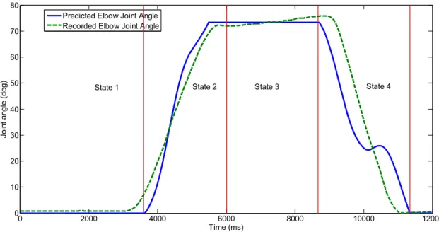
4.5 State switch algorithm ... 58
4.6 Experimental results ... 62
IX
4.6.2 Experimental results ... 65
4.5 Summary ... 73
Chapter 5 Force Evaluation and Prediction using sEMG 5.1 Introduction ... 75 5.2 Muscular model ... 76 5.3 Motion recognition ... 80 5.4 Parameter calibration ... 81 5.5 Experimental results ... 83 5.5.1 Experimental setup ... 83
5.5.2 Experimental results for motion recognition ... 86
5.5.3 Muscle activation during force exerting ... 88
5.5.4 Parameter calibration ... 90
5.5.5 On-line experimental results ... 93
5.6 Summary ... 96
Chapter 6 Entire System Evaluation 6.1 Introduction ... 99
6.2 System construction ... 99
6.3 Evaluation of self-training function ... 102
6.3.1 Schematic of self-training function ... 102
6.3.2 Experimental results ... 103
6.4 Evaluation of remote force evaluation function ... 109
X
6.4.2 Experimental results ... 111
6.5 Summary ... 118
Chapter 7 Concluding remarks 7.1 Thesis summary ... 121
7.2 Research achievement ... 123
7.3 Recommendations for the future ... 125
References ... 127
Publication List ... 141
XI
List of Figures
Figure. 1.1: Two type of recording method for EMG signals ... 5
Figure 2.1: The Upper-Limb Exoskeleton Rehabilitation Device ... 15
Figure. 2.2: Tele-operation system for rehabilitation training ... 16
Figure. 3.1: Change in AR model coefficients compared to amplitude trend in sEMG signals ... 22
Figure. 3.2: Plot of all-roots with equation (3-2) ... 23
Figure. 3.3: Value of the AIC algorithm to increasing of order p ... 25
Figure. 3.4: The classic structure of Neural Network ... 26
Figure. 3.5: sEMG signal recording system ... 31
Figure. 3.6: Experimental procedure A ... 33
Figure. 3.7: Experimental procedure B ... 33
Figure. 3.8: Experimental procedure C ... 34
Figure. 3.9: The confusion matrix of the performance ... 34
Figure. 3.10: BP ANN recognition results for volunteers with their own ANN and the other’s ANN ... 36
Figure. 3.11: The confusion matrix of the performance. ... 37
Figure. 3.12: Experimental results of features extracted by AR model ... 38
Figure. 3.13: Experiment of wrist adduction and abduction ... 44
Figure. 3.14: On-line testing performance with MM feature extraction method ... 46
XII
Figure. 3.16: Time consumption for on-line testing process... 48
Figure. 4.1: Three-element Hill-type muscular model ... 52
Figure. 4.2: Musculoskeletal model of elbow joint ... 54
Figure. 4.3: Muscle activation levels compared with elbow joint angles ... 59
Figure. 4.4: Schematic of state switching method ... 61
Figure. 4.5: On-line experiment of controlling a virtual arm ... 64
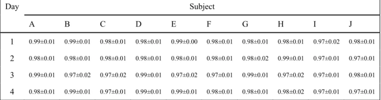
Figure. 4.6: Model validation results of the ten subjects ... 66
Figure 4.7: Experimental results of continuous elbow joint angle prediction method ... 68
Figure. 4.8: Time lag in real-time caused by state switch algorithm. ... 70
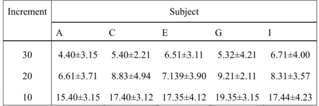
Figure. 4.9: Consecutive stepping test results for different increment angles ... 72
Figure. 5.1 Downward touch motion ... 79
Figure. 5.2: Push motion ... 79
Figure. 5.3: One example of the push motion ... 81
Figure. 5.4: Gestures for the two motions ... 84
Figure. 5.5: Remote force evaluation experiment ... 85
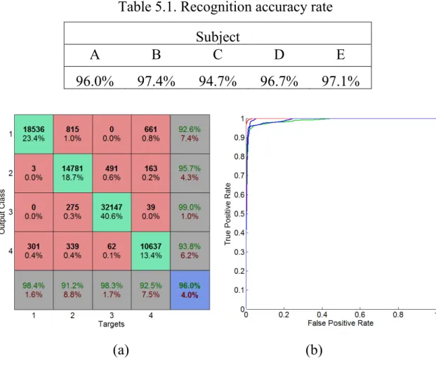
Figure. 5.6: Training performance of the Neural Network classifier from one subject ... 87
Figure. 5.7: On-line experimental results of motion recognition ... 88
Figure. 5.8: Muscle activation levels during contact force exerting ... 90
Figure. 5.9: Off-line force prediction results... 92
Figure. 5.10: ‘Cross-validation’ of two subjects ... 93 Figure. 5.11: On-line experimental results for downward touch force
XIII
prediction ... 96
Figure. 5.12: On-line experimental results for push force prediction ... 96
Figure. 6.1: Schematic of the entire project ... 100
Figure. 6.2: Schematic of the proposed system ... 101
Figure. 6.3: Schematic of the self-training function ... 102
Figure. 6.4: Subject with ULERD ... 103
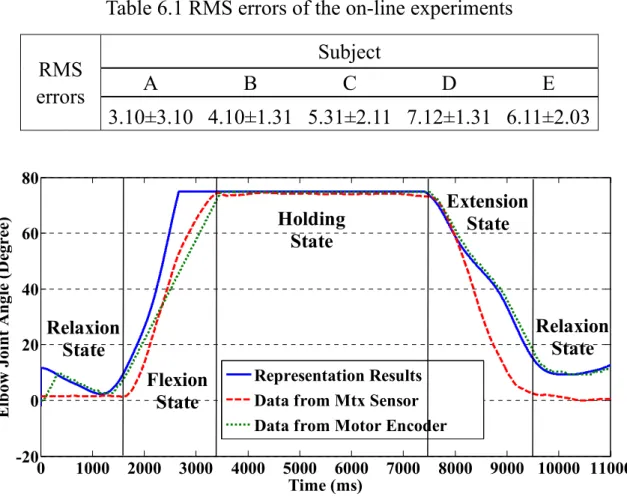
Figure. 6.5: On-line experimental results ... 104
Figure. 6.6: Experimental results of continuous movement ... 105
Figure. 6.7: Results with different order of Butterworth filter ... 106
Figure. 6.8: Experimental results of consecutive stepping test ... 108
XV
List of Tables
Table 3.1 Order P to AIC ... 25
Table 3.2 Accuracy of artifical neural network ... 34
Table 3.3 Accuracy of artifical neural network ... 36
Table 3.4. Performance of off-line training. ... 45
Table 3.5. Performance of on-line testing. ... 45
Table 4.1 Correlation coefficients between experimental data and proposed model ... 66
Table 4.2 Experimental results of the ten subjects ... 68
Table 4.3 RMS errors between prediction results and recorded results in consecutive stepping test ... 73
Table 5.1. Recognition accuracy rate ... 87
Table 5.2. RMS errors of on-line downward touching force prediction results ... 95
Table 5.3. RMS errors of on-line pushing force prediction results ... 95
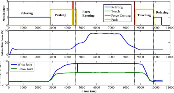
Table 6.1 RMS errors of the on-line experiments ... 104
Table 6.2 Force prediction for 5 N group with parameters calculated from 5 N group ... 111
Table 6.3 Force prediction for 10 N group with parameters calculated from 5 N group ... 112
Table 6.4 Force prediction for 15 N group with parameters calculated from 5 N group ... 112 Table 6.5 Force prediction for 5 N group with parameters calculated from
XVI
10 N group ... 114 Table 6.6 Force prediction for 10 N group with parameters calculated from 10 N group ... 115 Table 6.7 Force prediction for 10 N group with parameters calculated from 15 N group ... 115 Table 6.8 Force prediction for 5 N group with parameters calculated from 15 N group ... 116
1
Chapter 1
Introduction
1.1 Neurorehabilitation
It is reported by World Heart Federation that 15 million people worldwide suffer a stroke every year and nearly six million die and another five million are left permanently disabled [1]. Stroke is the second leading cause of disability, which wildly affects peoples’ Activities of Daily Living (ADL) and the life style of their families. As it has been stated that ‘Rehabilitation, for patients, is fundamentally a process of relearning how to move to carry out their needs successfully.’ [2], rehabilitation is such kind of training process therapists help patients to recover their function of movement as they used to be before stroke. Fortunately, some researchers [3] found that the neurons of some animals and humans are plastic, and the motor cortex functions can be altered by individual motor experiences. Some training strategies are developed based on this found, such as intensive intervention [4], task orientation training [5-7], bilateral training [8], electromyographical biofeedback [9], and functional electrical stimulation training [10], towards the function of neurorehabilitation. Although the neurorehabilitation itself is at the infancy stage and remains lots of challenges to researchers and doctors, the basic concept of neurorehabilitation that practice will improve the performance of motor learning is advanced in the rehabilitation topic [11]. Normally, these strategies require intensive, long duration and high-level training periods
2
[12] which will bring much burden to therapists.
1.2 Robots for rehabilitation
Robots have been implemented on rehabilitation since 1980s [13]-[15]. MIT-Manus [16],[17], ARMin [18]-[19],[84]-[85] and MIME [20]-[21] have been thought to be the pioneers for developing therapeutic robot systems for rehabilitation and reporting treatment results on patients. Rather than other fields’ requirements, more elaborate demands are needed to design robot systems for rehabilitation. Some literatures [22] divided these requirements into three aspects: psychological, medical and ergonomic. For psychological aspect, it is required that therapist and patient are both motivated. During the training process, the robot remains assistance or ‘invisible’ to the therapist and the therapist plays the main role for the patient. A ‘human-friendly’ design is also welcome for the psychological purpose [23]. For medical aspects, the robot should be adapted or adaptable to the human limb in terms of segment lengths, range of motion (ROM) and the number of degrees-of-freedom (DOFs). Although large DOFs may fit the patient well, it could make the device complex, inconvenient and expensive as well. No mention that it is still under discussion that whether large DOFs is good for rehabilitation or not. For ergonomic aspects, the rehabilitation robot set-up must be rather flexible to cope with a large variety of different applications and situations. The device should be suitable for different body heights and weights or gender.
Robots can provide more intensive, longer duration and higher-level training than therapists. A well programmed, backdrivable robot can
3
achieve active interactive training effort for patients. The impedance controller, which is introduced by Hogan [24], is widely used for the purpose of robotics and human-system interaction. Lum et al [20] developed the mirror image enhancer (MIME) arm therapy robot. The affected arm performs a mirror movement of the movement defined by the intact arm. The MIME can provide four different control models for patients. The virtual reality (VR) concept is also applied on rehabilitation [25]-[27]. This kind of system can mimic the real ADLs environment to enhance the activation for central nervous system.
1.3 Electromyography signals
As mentioned in section 1.1 that the electromyography (EMG) biofeedback technology is also applied on rehabilitation.EMG signals are detected when skeletal muscles are activated by the center nervous system. When activation comes from the nervous systems, action potential is achieved on membranes of muscle fiber cells in one motor unit. This excitation, which spreads along muscle fiber in both directions and inside muscle fiber through a tubular system, releases calcium ions in the intra cellular space [28]. Linked chemical processes finally shorten contractile elements of the muscle cell. Raw sEMG signals, which are detected through electrodes placed on the skin of the upper limb, are superposition of different Motor Unit Action Potentials [29] (MUAP). The two most important mechanisms influencing the magnitude and density of the observed signal are the recruitment of MUAPs and their firing frequency.
4
kind of biological signals can be used for interpretation of muscle activation levels. Methods used for nowadays are very simple and direct to obtain muscle activation level from EMG signals. One of the simplest ways is to normalize the EMG signal by dividing it by the peak rectified EMG value obtained during a maximum voluntary contraction (MVC). This method may be the most conventional one for the researchers around the world to process EMG signals. Still it is open for discussion that whether it is appropriate to just use this simple way to obtain muscle activation level. Some researchers suggested that a more detailed model of muscle activation dynamics is warranted in order to characterize the time varying features of the EMG signal. One of such kind of model or method is called Discretized Recursive Filter (DRF) [30]. This method is based on the phenomenon that when a muscle fiber is activated by a single action potential, the muscle generates a twitch response. A damped linear second-order differential system can well represent this response and the DRF is just the discrete equation which describes this differential system. Although a linear approximation of muscle activation from EMG signals seems reasonable and suitable, the activation is nonlinearly related to EMG in many cases. Some equations [31]-[33] have been established based on the nonlinear concept.
1.4 Implementation of EMG signals
According to the different measurement method, EMG signals can be divided into surface ones, which are recorded by electrodes attached on the skin above the target muscle belly, and intrinsic ones, which are recorded
by re an su F 1. si ad m am fa fo se L y needles ecorded E natomical urface EM Figure. 1.1 one rec .4.1 Utiliz Predic ignals. Fuk dopted a mixture ne mong ind atigue or s or the man ense a fee Liarokapis inserted i EMG sig and medi MG or sEM (a) 1: Two typ orded by n zation of E ction of m kuda et al statistical etwork, to dividuals, sweat. The nipulator a eling of p et al. [35] into the m gnals. As ical knowl MG is wide pe of recor needle [81 EMG motions m . [34] used l neural n o achieve electrode ey reported and it mig prosthetic ] used EM 5 muscle fibe s using ledge and ely used fo rding meth 1]; (b) sho electro may be th d EMG sig network, n e robust s location d that the ght allow control s MG signals -0.25 -0.2 -0.15 -0.1 -0.05 0 0.05 0.1 0.15 0.2 V ers. Fig 1 the need it may br for enginee hod for EM ows the on de. he most p gnals to co named the discrimin ns, and ti method c a physica imilar to s from six 0 2000 4000 5 2 5 1 5 0 5 1 5 2 .1 shows dle requir ing pain to ering purp (b) MG signal nes recorde opular ap ontrol a m e log-line nation aga ime varia an provide ally handic that of th xteen musc 6000 8000 1 Time (ms) the two k res profe o the subj poses. ls. (a) sho ed by surf pply with manipulato earized G ainst diffe ations cau de smooth capped pe he origina cles of the 0000 12000 14000 kinds of essional ect, the ws the face sEMG or. They aussian ferences used by control erson to al limb. e upper 16000
6
limb to study the muscular co-activation patterns during a variety of reach-to-grasp motions. Artemiadis et al. [36] developed a switching regime model to decode the EMG activity from 11 muscles into a continuous representation of arm motion in three-dimensional space. Ju et al. [37] designed a fuzzy Gaussian mixture model with non-linear feature extraction method to classify different hand grasps and in-hand manipulations. They reported that using their proposed non-linear method the highest recognition rate of 96.7% could be achieved. This kind of implementation is very meaningful for control of prostheses or robot arms intuitively. The operator doesn’t need the control panel anymore but just performs his/her accustomed motions to control the device. Besides pattern recognition based methods, some researchers also proposed continuous prediction method. Earp, et al. [98], proposed a polynomial relation between EMG signals and knee angles. Vogel, et al. [99], recorded the EMG of atrophic muscles to control a robot arm continuously. Alternatively, An, et al. [100], offered a muscle synergy based method to mimic the human standing-up motion by recording EMG signals from lower limbs.
Another implementation is to use sEMG signals to calculate musculotendon forces [87-91]. Actually, besides the muscle activation level, the musculotendon force is the most direct one that EMG signals reflect. As the activation signals to muscle contraction, the EMG signal certainly has a strong relationship with musculotendon forces. Two physiological models are widely used for musculotendon forces prediction: Huxley- [38,39] and Hill-type models [40]. Compared with the complexity of Huxley-type
7
models, Hill-type models are more computationally viable. Cavallaro et al. [41] developed a Hill-type-model-based myoprocessor to predict joint torque. Seven muscles around the upper limb were recorded and a genetic algorithm was implemented to tune the parameters of the model. Manal et al. [42] used a Hill-typed model to calculate muscle force and implemented a forward dynamics approach to estimate joint angle. They used an optimal controller to map the relationship between measured and predicted joint moments. Fleischer and Hommel [43] used the sEMG signals and Hill-type based biomechanical model to control a lower-limb exoskeleton device. It should be noticed that the EMG signal is not the only one involved in the muscular model. For example in Hill-type model, the EMG signal is used to reflect the muscle activation level which is just one of the variables in the function, together with other hard to be measured ones, such as muscle changed length, changing velocity and the status of the tendon. Hogan also discussed the function of coactivation of antagonist muscles to maintain the posture of the forearm and hand [86].
Besides motion recognition and musculotendon force prediction, EMG signals are also applied on controlling of force enhance or power assistance system [95-97]. Lenzi et al. [44] proposed a simple sEMG signals based powered exoskeleton control method that can support the subject depending on the amplitude of detected sEMG signals. They reported that such kind of simple proportional control method can provide suitable results for their particular purpose. Kwon et al. [45] gave an analysis on the stability of sEMG-based elbow power assistance. They
8
wanted to set up a foundation for determining the appropriate amount of such kind of device. Moreover, some researchers used sEMG signals to perform impedance control. Ajoudani et al. [46] proposed a tele-impedance body-machine interface to perform a peg-in-the-hole and a ball-catching task. The sEMG signal was used to predict the stiffness of the operator’s arm and a stiffness variable robot arm was applied to reflect the predicted stiffness.
1.4.2 Issues of EMG
Despite the attractive application of EMG signals on various fields, the EMG signal is still hard to be used outside the laboratory environment. Time-variable, non-stationarity, low signal-to-noise ratio, individual differences, and easily affected by external factors [92-94] become the primary factors that give rise to the ‘hard-to-use’ property of EMG signals.
As the complexity of mechanism of muscle activation procedure and the human musculoskeletal system, EMG signals seems non-linear and time-variable to every interesting targets, such as musculotendon force, to-be-predicted motions or stiffness of limbs. Compared with non-linear, the time-variable makes the problem even worse. For the same desired target or behavior, EMG signals change wildly and frequently. It is hard or impossible to find the exact mapping between EMG signals and the target. It seems like that a random noise is always added on the original EMG signals, which may be the reason that why researchers tend to apply machine learning algorithm to solve the problem concerned with EMG signals. Chen et al. [47] developed a multi-kernel learning support vector
9
machine method to classify multiple finger movements. In order to recognize hand motions, Tang et al. [48] applied a multi-channel energy ratio feature extraction method to overcome the influence of various forces for a given gesture. They used the proposed feature extraction method and a cascaded-structured classifier to recognize eleven hand gestures. Phinyomark et al. [49] implemented twelve anthropometric variables to design an automatic/semi-automatic calibration system for EMG recognition. Although many elegant algorithms have been developed [50-52], you still cannot treat this biological signal as the one obtained from conventional sensors, such as a force sensor or a position sensor.
For the low signal-to-noise ratio (SNR) aspect, Clancy [53],[54] proposed a time-varying selection of the smoothing window length method and white noise preprocessing method to improve SNR of EMG signals. The use of different cut-off frequency filters are also suggested by researchers [55]. Although this issue seems less important with the growing of signal processing technology, the researchers are still disturbed by the SNR problem, caused by inevitable factors, such as crosstalk.
1.5 Thesis contributions
In this thesis, a home-used upper-limb rehabilitation system was proposed, focusing on characteristic evaluation and the control method development.
Contributions of this thesis are:
(1). Development of bilateral self-training function using ULERD and sEMG signals.
10
The bilateral self-training function aimed to release the burden from therapists. Although the supervising from therapists is necessary for patients, for hemiparesis patients, they need training practice frequently at home in most of the time. In the proposed system, the patient is asked to wear the ULERD on his/her impaired upper-limb and electrodes are attached on the intact upper-limb. Then the patient is asked to perform training exercise bilaterally. The control reference is obtained from sEMG signals obtained from the intact upper-limb. One of the advantages of this system is that patient can guide by himself using the intact limb. Although it is still being studied, the research results indicate that positive exercise which is activated by Centeral Nervous System (CNS) or the willing of patient is more effective than passive exercise which is carried out by therapists or devices. Another advantage is that the control reference is obtained from the EMG signal. Rather than the conventional motion signals, such as angle value or trajectory obtained from motion capture system, the EMG signal reflect the intention of the motion and it is the original signal reflect the activation from CNS.
(2). Evaluation of motion to sEMG signals. A motion recognition method and a continuous elbow joint angle prediction method were proposed.
In order to map the sEMG to motions, a motion recognition based method was proposed firstly. The wavelet packet transform was applied to remove the influence from noise and a muscular model was used to extract features. Compared with conventional signal processing method, the muscular model based model reflects more natural property of the sEMG
11
signals. For classifier, the support vector machine (SVM) was chosen to recognize motions. In our particular cases, the SVM is more robust than the neural network classifier. Nevertheless, the motion recognition method has its own limit. It can only provide binary-like control reference, but in many cases, continuous prediction results are needed. For the purpose of providing continuous prediction results, a musculoskeletal model based elbow joint angle prediction method was proposed. A quadratic relationship was derived from the musculoskeletal model and Hill-type based muscular model. A state switching function was developed to conquer the problem of time-variable characteristic of sEMG signals. The proposed method can predict elbow joint angle continuously using only EMG signals.
(3). Development of human-environment contact force prediction method. Another function of the home-used upper-limb rehabilitation system is that it can provide remote force evaluation. The force prediction is achieved by using only sEMG signals. To use sEMG signals can avoid the inconvenience of attaching force sensor and constrain of the motion of patients. Two isometric motions are focused on in this thesis, namely downward touch motion and push motion. Two dynamic equations were derived from the two motions, respectively. The parameters involved in the two equations were calibrated by Bayesian Linear Regression (BLR). The application of BLR can avoid the problem of over-fitting and the natural property of BLR treats the issue on the probability point of view which solves the problem of time-variable for sEMG signals. A haptic device ‘Phantom Premium’ was used to represent the predicted force on the
12 remote side.
13
Chapter 2
Motivation and Research Purpose
2.1 Motivation
Although many robotic rehabilitation systems have been developed since 1980s, home-used robotic rehabilitation systems are seldom seen. Large robotic systems are just suitable to be used in rehabilitation center for special purpose and under the supervision of therapists. Consider the amount of patients needed to be treated and the number of robotic systems being used, there is still a long way to go for the popularization of robotic system in rehabilitation training. On the other hand that the mild stroke patients don’t quite need the medical treatment using such kind of large robotic system. Usually these patients are asked to perform rehabilitation training by themselves, with some simple assistance devices, and under the supervision of their families. In most of the cases, these patients are lack of supervision from the therapist and are not well motivated, as the families members are not well trained on concept of rehabilitation. With time going on, they may lose interest and feel bored for rehabilitation training. As a consequence, the training intension and duration is not enough to achieve a good result. And lacking of supervision from the therapist may lose some good opportunities for a better training timing.
It can be indicated that there are huge demand of relative small home-used robotic rehabilitation system. This kind of rehabilitation system should be small enough to be portable, to be able to provide active or
14
passive training assistance as needed and to be able to provide evaluation method to observe the status of patients. A remote function may be more attractive because it will save the time wasted on the road to rehabilitation center and waiting for the therapist. Furthermore, on the neurorehabilitation training point of view, just simple movement of the impaired limb is not good enough for rehabilitation. The patient should be inspired to perform the movement under his/her own will, i.e. under the command from CNS. The experimental results from Lum et al. [8] indicated that a ‘bimanual mode’ or bilateral training strategy will inspire the patient well. The bilateral type of rehabilitation may be helpful for patients to complete the training exercise at home. On the other hand, it will be also a useful function that the rehabilitation system can provide remote evaluation for the therapist to supervise the patients.
2.2 Upper-limb exoskeleton rehabilitation device
In our previous study, an Upper-Limb Exoskeleton Rehabilitation Device (ULERD) (as shown in Fig. 2.1) has been designed [56-59]. The total weight of ULERD is 1.3 kg which is light enough for portable purpose. It has seven DoFs, including three active DoFs (one for the elbow joint and tow for the wrist joint) and four passive DoFs (two for the elbow joint and two for the wrist joint). The passive DoFs aimed to achieve the requirement from ergonomic aspect as mentioned in section 1.2. This device can provide active training, in which a resistant force will be exerted on when patient performs rehabilitation exercise. The function is achieved by impedance control algorithm. Besides, a passive training model can also be
se or re w (a
2
sh w in ap ex elected, in rder from The U ehabilitatio wear the d active and Figur.3 Devel
We al hown in F wears the U n the prop ppeared b xecuted b n which t a supervis ULERD p on system device to passive) a re 2.1: Theloped Tel
lso develo Fig. 2.1) t ULERD on posed train block disp y patient he device sor. provide a m. The we perform are suitabl e Upper-Lle-opera
oped a si to inspire n the impa ning exerc played on and thera 15 e will carr a hardwar eight is li the ADL le to fit th Limb Exosation syst
imple tel patient. In aired arm cise is to n the scre apist toge ry the im re founda ght enoug Ls and the he various skeleton Rtem for r
e-operatio n the tele and holds control a een. The o ther. A sp mpaired arm ation for gh to allo e possible needs from Rehabilitatirehabilit
on interac -operation s a haptic a beam to operation pring-dam rm follow the hom ow the pat e driven m patients tion Devictation
ction syst n system, device. T o track a r of the b mping mod ing the me-used tient to models s. ce em (as patient The task random beam is del was16
designed for the operation. The system will provide assistance or resistance force to the patient via the haptic device and our ULERD. The exercise can be controlled by therapist on the remote side. The idea for this tele-operation system is that the training exercise can be performed by tele-operation, not required the therapist to be at present to supervise the training. The detailed information for this system can be found in [82, 83].
Figure. 2.2: Tele-operation system for rehabilitation training
2.3 Research purpose
The purpose of this thesis is to propose a home-used upper-limb rehabilitation system including the following properties:
17
to provide self-training to the patient. The self-training should follow the concept of bilateral exercise from the neurorehabilitation point of view. (2) To realize remote evaluation, a force prediction method should be developed. The method should reflect the status of the patient as entirely as possible. For such purpose, the force sensor may not be enough, because it can only reflect the end-effect performance of the patient.
(3) As one of the state-of-the-art technologies to control prostheses or robot arms, it is necessary to evaluate the relationship between sEMG signals and kinetics variable of human. A dynamic equation, if possible, is desired to interpret the relation between sEMG signals and motions.
Additionally, a deeper understanding of the relationship between human and exoskeleton device, e.g., how to improve the control interaction, how to improve the control algorithm to fit device better for subject, will be desired to release via the research.
19
Chapter 3
Motion Evaluation and
Recognition using sEMG
3.1 Introduction
Using sEMG to recognize motion of human is one of the most prominent applications of this biological signal for engineering purpose. It is extremely useful toward intuitive control of prostheses or robot arms. The patient who loses his/her arm in an accident can mount the prostheses on the remaining part of the wounded arm and control signals will be extracted from sEMG signals recorded from the remaining muscles. In this way, the patient will feel like that controlling the prostheses is just like the original arm [34]. Some commercial products [60-62] have been developed towards this kind of application. These products are capable of performing complex motions by integrating more electrodes or sensory feedbacks. Furthermore, it has to be said that the remaining muscles may have no relationship with the target motions, depending on the wound situation. Under such circumstance, the patient, actually, uses an alternative way to perform the motion, i.e. using another group of muscles, because of lack of the original ones. However, it is still advanced than pushing bottoms on a control panel to control the prostheses.
From the neuromechanics point of view, human motion is just the output of CNS and musculoskeletal system. The EMG signal is a little previous than the measured movement (about 30 to 100 ms, namely
20
electromechanical delay (EMD) [63]). The existence of EMD indicates that it is theoretically possible to predict motion using EMG signals, which will bring much advance to control method.
In this chapter, the evaluation between human motion and sEMG signals will be discussed, and a motion recognition method will be introduced. Upper-limb motions, which include elbow flexion and extension, forearm pronation and supination, wrist flexion and extension, and adduction and abduction, are mainly focused on. These motions are involved in ADLs commonly. An autoregressive (AR) model based feature extraction and neural network based classification method will be introduced firstly, followed by an improved Hill-type muscular model based feature extraction and support vector machine (SVM) classifier recognition method.
3.2 Design of motion recognition method with neural network
3.2.1 Autoregressive based feature extractionTo extract features of sEMG signals, an autoregressive (AR) time series model is applied in this thesis [65]. The AR model was introduced in the study of EMG signals in 1975, when Graupe and Cline first used this model to represent electrical muscle activation behavior [64]. In statistics and signal processing, the AR model is a type of random process that is often used to model and predict various types of natural phenomena. Because EMG is a random natural signal, it is very suitable to use the AR model to extract features. The AR model is defined as follows
21
where is the order of the AR model, Xt is the value of data, φi is coefficient, c is a constant and εt denotes the white noise.
For original purpose of the applying AR model, which is to predict output of a system based on previous outputs, it is reasonable to consider that coefficients (φi) of the model are representative of the sequence of input data or the model itself is capable of catching feature from the raw data. Fig. 3.1 provides some calculation results using the Burg method [78] to fit raw sEMG signals detected from biceps brachii with a 4th order AR model, where the above red line denotes the second coefficient of the AR model, and the below blue line represents for the raw sEMG signals. The upper line in Fig. 3.1 was calculated with a time interval of 50 ms (sampling frequency of 1000 Hz). The results show that changes of the coefficient follow the trend in sEMG signals. Additionally, it should be noticed here that this kind of phenomenon gave us the idea that whether we could find some way to extract the trend from the EMG signals to map the motion. The different sequences of coefficients represent different sequences of raw signals. For example, coefficients in Fig. 3.1 from time intervals 1 to 10 stand for raw signals from 1 to 500, coefficients from 11 to 25 stand for signals from 550 to 1250, coefficients from 26 to 40 stand for signals from 1300 to 2000, and so on. As the sEMG signals were recorded from the motions continuously, different sequences of the coefficients of the AR model are consequently representative of the different motions of the upper limb. So in this thesis, coefficients of the AR model are divided following different motions of the upper limb and then grouped coefficients
22
are used as input to the neural networks for pattern recognition.
Time consumed by AR model is low, and it is suitable in real-time calculation. sEMG signals were calculated using the AR model in real time with a certain time window (with 50 ms in this thesis), and then coefficients of the AR model are used as input to a well-trained neural network. The time consumption for the entire procedure was about 50 ms, as the time interval used for AR model computing was 50 ms and time consumption for motion recognition was only around 0.03 ms.
Figure. 3.1: Change in AR model coefficients compared to amplitude trend in sEMG signals [77]
There are two primary parameters in the AR model. One is the interval of the time window (t) used for data calculation and the other is the order (p) of the AR model.
There is the constraint that the AR model requires that predicted data be wide-sense stationary. It has been indicated that raw sEMG signals are
23
nonstationary [64], but with sufficient short time intervals, this nature of electrical behavior could be considered stationary. It is thus important to select a suitable processing time window when using the AR model in extracting the features of the sEMG signal. In order to judge the appropriateness of time intervals, all of the roots of polynomials, as described in equation (3-2), must lie within the unit circle in complex plane.
x + ∑ φ x = 0 (3-2) For this study, raw sEMG sequences were divided into 50 ms ( each 50 samples at a 1000Hz sampling rate) intervals and the following figure shows calculation results using equation (3-2), where the circle represents the unit circle:
24
Fig. 3.2 shows that all of the roots are in the unit circle, which means that all of the AR models remain wide-sense stationary.
It is also necessary to determine the optimal order before using the AR model fitting the sEMG signal. If the order is too small, the fitting effect will be so weak that the recognition accuracy rate will be adversely affected. Because in such condition, the feature losses the representation property for the sEMG signals and tends to be the signals themselves. As the consequence of the low signal-to-noise ratio characteristic of sEMG signals, the classifier can hardly convergence with such kind of training data. If the order is too big, however much computation time will be required, which will influence the real-time control effect as well.
To guarantee a suitable order, the Akaike Information Criterion (AIC) [79], which is a well-known criteria, was used as the judgment criterion. The following equation describes the AIC algorithm:
AIC(p) = ln (E ) + 2(p + 1)/N (3-3) where Ep is the estimated linear prediction error variance for the model with order p and N is the number of input sEMG signals. The order that minimizes the AIC function results is selected as the optimal one.
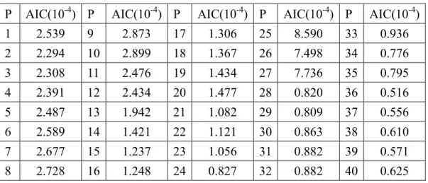
The result of the AIC method is represented in Table 3.1 with AR model order P from 1 to 40, and Fig. 3.3 describes the general trend of change.
25
Table 3.1 Order P to AIC
P AIC(10-4) P AIC(10-4) P AIC(10-4) P AIC(10-4) P AIC(10-4)
1 2.539 9 2.873 17 1.306 25 8.590 33 0.936 2 2.294 10 2.899 18 1.367 26 7.498 34 0.776 3 2.308 11 2.476 19 1.434 27 7.736 35 0.795 4 2.391 12 2.434 20 1.477 28 0.820 36 0.516 5 2.487 13 1.942 21 1.082 29 0.809 37 0.556 6 2.589 14 1.421 22 1.121 30 0.863 38 0.610 7 2.677 15 1.237 23 1.056 31 0.882 39 0.571 8 2.728 16 1.248 24 0.827 32 0.882 40 0.625
Fig. 3.3 shows that the trend of the AIC value decreases gradually although there is a small increasing trend during orders 2 to 10. From orders 10 to 15, there is a distinct decrease from 2.899x10⁻⁴ to 1.237x10⁻⁴, and from 16 to 40, the decrease is not very overt. Considering calculation time cost, 15 was selected as the optimal order for the AR model at this time.
26
3.2.2 Neural network as classifier
Before starting this section, I have to state that this section is just going to introduce the neural network classifier which I used and the consideration of using thus kind of classifier. There is no new point on the algorithm or network structure, as it is not my research focus to find a more effective and optimal neural network but looking for the relationship between sEMG signals and pattern recognition methods.
The term of ‘neural network’ is derived from the study of attempting to find mathematical representations of information processing in biological systems, for instance the human brain [66]-[68]. A mathematical function description for the neural network is:
1 1 1 1 2 1 1 1 1 1 1 2 1 1 1 1 1 ( ( n (... ( )))) n n n D D M n n n n kj ki ji i i i j i i y
σ
ω
h −ω
h hω
x − − − − − − = = = =∑
∑
∑
(3-4)where σ is the output layer activation function and hn-i is the activation function of the hidden layer. The superscript n-i denotes the corresponding layer. ω represents the parameters which needs to be adjusted. xi is the input for the neural network and y is the output. The diagram of such a neural network is plotted in Fig. 3.4.
27
The information flow in such a network structure is forward, from one layer to the next layer, and a network with such kind of structure is called feed-forward networks. The selection of the activation function for each layer is various, such as linear, logistic sigmoid and ‘tanh’ function. One property of feed-forward networks is that multiple distinct choices for the parameters of ω can lead to the same mapping function from inputs to outputs [69], which is called weight-space symmetries.
In most of cases, the training process is divided into two stages: the first one is to derivate the error function with respect to the parameters or weights; and the second one is to use the derivatives calculated in the first stage to compute the adjustments to be made to the weights. In the first stage, the error backpropagation algorithm is used to obtain a computationally efficient method for evaluating derivatives. And this is the very reason that such kind of network is called backpropagation neural network. And for the second stage, the conjugate gradients are widely adopted.
The steps for error backpropagation are:
(1) Apply an input vector x to the neural network and forward propagate to find the activations of all the hidden and output units of layers.
(2) Evaluate the δk for all the output units using equation 3-5:
= − (3-5) (3) Backpropagate the δ using equation 3-6 to obtain δj for each hidden unit.
28
(4) Use equation 3-7 to evaluate the required derivatives:
= (3-7) The steps for the scaled conjugate gradient algorithm are [72]:
(1) Choose arbitrary parameters of scalars σ>0, λ1>0 and λ’1=0. Set p1
= r1 = -E(ω1) and a variable flag success = true.
(2) If success = true then used the derivatives calculated in the error backpropagation process: = | | (3-8) = ( ) ( ) (3-9) = (3-10) (3) Scale sk: = + ( − ) (3-11) = + ( − )| | (3-12) (4) If δk ≤ 0 then make the Hessian matrix positive definite:
= + ( − 2| | ) (3-13) = 2( −| | ) (3-14) = − + | | , = (3-15) (5) Calculate step size:
= + ( − ) (3-16) (6) Calculate the comparison parameter:
Δ = ( ( ) ( )) (3-17) (7) if Δk ≥ 0 then a successful reduction in error can be made:
29
= + (3-18) = − ′( ) (3-19) = 0, success = true. (3-20) (7a) If k mod N = 0 then restart algorithm: pk+1 = rk+1
else create new conjugate direction:
=| | (3-21) = + (3-22) (7b) If Δk ≥ 0.75 then reduce the scale parameter:
= 0.5 (3-23) Else a reduction in error is not possible:
′ = , success = false (3-24) (8) If Δk < 0.25 then increase the scale parameter:
= 4 (3-25) (9) If the steepest descent direction rk ≠ 0 then set k = k+1 and go to step 2 else terminate and return ωk+1 as the desired minimum.
It should be noticed that the error function used for parameters calibration is not convex over weight space. This property leads to one of the disadvantage that a local minimum may be found by the backpropagate process rather than a global minimum one. And there may be many local minimum points. Finding a proper one strongly depends on the starting point or the initial status of the parameters which in many cases are selected randomly.
In this thesis, a two-layer neural network with one hidden layer and one output layer was adopted to be the classifier. The activation function
30
for hidden layer and output layer is hyperbolic tangent sigmoid transfer function. The number of neurons in the hidden layer is n+2 where n is the dimension of input vector and in this particular circumstance it equals the number of muscles used for sEMG signals recording. The output are vectors structured by one-of-k coding scheme where k is the number of patterns.
3.3 Experimental results with neural network
3.3.1 Experimental setupThree healthy volunteers aged from 22–26 years, all male, one left-handed and two right-handed, participated in the experiment. Before placing the electrode, which was aligned parallel to the muscle fibers, over the belly of the muscle, the skin was shaved and cleaned with alcohol in order to reduce skin impedance. The sampling rate was 1000 Hz with differential amplification (gain: 1000) and common mode rejection (104dB). A fourth-order high-pass Butterworth filter with a 10-Hz cut-off frequency was implemented in software to remove the DC offsets in EMG signals before they were rectified. The user interface was programmed using Visual C++ 2010 (Microsoft Co., USA). The analog/digital (A/D) data from the A/D board was collected through the application programming interface and processed with MATLAB (The MathWorks Co., USA). The software was run on a personal computer with a 2.8-GHz quad-core processor (Intel Core i7 860) and 4 GB of RAM. Two MTx sensors (Xsens Technologies B.V., USA) were attached on the subject’s forearm and hand to record the elbow joint angle and wrist joint angle,
31
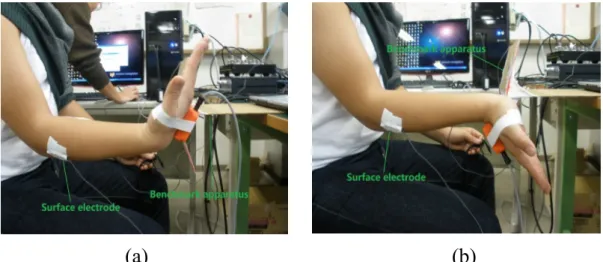
respectively, for calibration and comparison. Dry rectangle electrodes (Ag/AgCl, size: 26x14 mm), with a skin contact surface of 20 mm2, and inter-electrode distance of 18 mm, were placed parallel to the muscle fibers, according to SENIAM references [70]. Electrode placements were confirmed by voluntary muscle contraction and followed the recommendation of [71]. The apparatus used in the experimental are shown in Fig. 3.5.
(a) (b)
(c) (d)
Figure. 3.5: sEMG signal recording system. (a): personal EMG filter box; (b): surface electrodes; (c): Profile of the MTx inertial sensor; (d): AD
32
The motions to be recognized are elbow flexion and extension, forearm pronation and supination, wrist flexion and extension, and wrist adduction and abduction. In order to generalization the upper-limb movement of the volunteers, their motions were restricted as requirement directing by a video. In the experiment of upper arm flexion and extension, the volunteer were asked to sit on a chair started with upper limbs relaxed vertically fitting to the vertical pillar of the benchmark apparatus (as shown in Fig. 3.6 a) and then contracted their experimental upper forearm to the horizontal beam (as shown in Fig. 3.6 b). After a short stop keeping the forearm to the horizontal position, the volunteer was asked to extend the forearm to the initial vertical position. In the experiment of forearm pronation and supination, the upper arm kept vertical and volunteer only pronated with his forearm, keeping the upper arm still. There is a cross mark on the ground to be the benchmark for pronation and supination (as shown in Fig. 3.7). In the experiment of palmar flexion and dorsiflexion, volunteer kept his forearm horizontal and flexed or dorsiflexed to the contracted bounds (as shown in Fig. 3.8). The movements are divided into two groups. In the first group, only elbow flexion and extension is focused. Motion patterns are elbow flexion, elbow holding, elbow extension and relaxing, i.e. there are four motions in the first group. In the second group, motion patterns are corresponded to the five main motions: elbow flexion and extension, forearm pronation and supination, wrist flexion and extension, and wrist adduction and abduction.
33
relaxation of one minute in every five tests. The raw sEMG signals were recorded separately from the three experiments and a special BP neural network coordinate to one experimenter would be trained using the collected data from the ten times repeated tests. After all the three volunteers finished their experiments, there were three independent neural networks belong to the different experimenters. The movement of each volunteer had been recognized with their own neural networks and the results were applied to the multi-motion recognition.
(a) (b)
Figure. 3.6: Experimental procedure A. (a): The start position of the experiment; (b): the vertical position when subject tries to hold his forearm
(a) (b)
Figure. 3.7: Experimental procedure B. (a): The forearm pronation; (b) the forearm supination.
34
(a) (b)
Figure. 3.8: Experimental procedure C. (a) The palmar flexion; (b) the palmar dorsiflexion or extension
3.3.1 Experimental results
The experimental results for the first group are listed in Table 3.2. The confusion plots for the three subjects are shown in Fig. 3.9, respectively.
Table 3.2 Accuracy of artifical neural network Subject A B C Recognition
rate 81.5 82.1 94.6
(a) Volunteer A (b) Volunteer B (c) Volunteer C Figure. 3.9: The confusion matrix of the performance
35
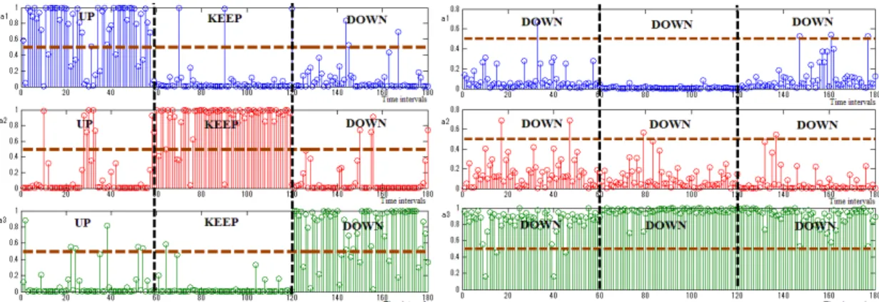
Recognition results for each volunteer with his own neural network and with the others are presented in from Fig. 3.10 a to c, where three different colors of dots stand for the three parameters in the result vector and the horizontal lines of dashes are critical dividing lines by which all of the data is separated into ones and zeros. The result vector is described as follows, where the standard result for up, holding, down and relaxing movement is (1, 0, 0, 0), (0, 1, 0, 0), (0, 0, 1, 0), and (0, 0, 1, 1) respectively.
(a). Recognition rate of volunteer A with his own ANN (the left) and with volunteer B’s ANN (the right)
(b). Recognition rate of volunteer B with his own ANN (the left) and with volunteer C’s ANN (the right)
36
(c). Recognition rate of volunteer C with his own ANN (the left) and with volunteer A’s ANN (the right)
Figure. 3.10: BP ANN recognition results for volunteers with their own ANN and the other’s ANN [65]
As shown at left in Fig. 3.10, results were calculated on line, and were used as reference input for motor control of the ULERD. As shown in Fig. 3.10 (c), from time intervals 1 to 60, almost all of the dots in group a1,
which represents a1 in equation (10), are positioned above the horizontal
line. After normalization using a piecewise function defined in (11), these parts of data equaled 1. In contrast, dots in group a2 and the dots in group a1,
are positioned below the horizontal line, equaled 0., These parts of recognition results consequently represented the vector of (1, 0, 0), which means the motion of the upper limb up.
The experimental results for the second group are listed in Table 3.3. The confusion plots for the three subjects are shown in Fig. 3.11, respectively.
Table 3.3 Accuracy of artifical neural network Subject A B C Recognition
37
(a) Volunteer A (b) Volunteer B (c) Volunteer C Figure. 3.11: The confusion matrix of the performance.
For the first group experiment, Biceps Brachii (BB) and Triceps Brachii (TB) muscles were chosen to record sEMG signals. As this pair of agonist and antagonist muscles take the main charge with the function of elbow flexion and extension, it is reasonable to choose this pair of muscles to study the movement of the elbow joint. Because the motion was performed in sagittal plane, TB was seldom activated. Furthermore, the involved movement includes concentric contraction motion (elbow flexion), isometric contraction motion (elbow holding) and active shortening motion (elbow extension). The muscle status is different among these motions. The behavior of EMG signals is different according to the different status of muscle. From this aspect point of view, the AR model used here is to extract features which represent the status of muscles as well. One set of the experimental results for AR model feature extraction is depicted in Fig. 3.12. The coefficients were calculated by Burg algorithm.
38
Figure. 3.12: Experimental results of features extracted by AR model As there are 15 features in AR model, only five of these parameters are plotted in the above figure. It can be indicated, although not very distinctly, that the changes of features are correspond with the changes of elbow motion. However, this kind of change decreases with the increasing of order.
3.4 Improved recognition method
The Neural Network is not an ultra remedy for all the issue of classification, much less that the Neural Network itself has many trouble issues. On the other hand, any of the existing classifiers will lose their function if the features themselves are not separable. It can be indicated from the experimental results in 3.3.1 that the feathers extracted by AR model are not stable or distinct. Another problem is with the Neural Network that it needs many times to train in order to get a proper classification performance. As it is also mentioned that to improve the feature extraction method and classifier algorithm is the key factor for
0 50 100 150 200 250 300 350 -2 -1.5 -1 -0.5 0 0.5 1 Sampling Times Value
39 motion recognition.
3.4.1 Support vector machine
SVM is proposed as a classification technique based on maximizing the margin between a data set and use optimal hyper plane to separate different data sets [72]. Compared with Neural Network, the advantage of SVM is that the target parameters depend on finding the optimal solution for a convex optimization problem, which is described as:
2 1 ( , ) 0.5 l i i c ϕ ω ξ ω ξ = = +
∑
(3-26) subject to [( ) ] 1 , 1, 2,..., i i i y x ⋅ω + ≥ −b ξ i = l (3-27)where x is an n-dimensional vector and b is a scalar. c is the independent variable. l is the number of data points. y is the model to be learned. (3-26) and (3-27) can be rewritten in the dual Lagrangian form:
1 1 1 ( ) l n 0.5 l l n m n m ( ,n m) n n m L a a a t t k x x = = = =
∑
−∑∑
a (3-28)where k(xn,xm) denotes the kernel function which plays the soul role in SVM. To classify new data using the trained model, (3-29) is used based on the conception of kernel function:
1 y( ) N n n ( , )n n a t k x x b = =
∑
+ x (3-29)where N denotes the number of support vectors.
40
quadratic programming problem in M variables in general has computational complexity that is O(M3). Considering that if there are 10,000 samples, which are just the number of variables in a quadratic programming problem, and each sample takes a 4-byte float type memory, a total 3725 GB memories are needed for computation. Fortunately, there is a popular approach to training SVM, which is called sequential minimal optimization (SMO) [73]. It is not until the discovery of the effective training algorithm that SVM has acquired a wide attention.
3.4.2 Improved feature extraction methods
It is intuitive to extract the trend of the EMG signal or finding some corresponded curve with low changing frequency to represent the changing for feature extraction.
A Weight Peaks algorithm was designed based on the above concept. The purpose of WP method is to try to catch the trend of original sEMG signals [74]. The reconstructed sEMG signals processed by WPT have the different frequency in different nodes. Therefore, the amount of peaks obtained in different nodes is different. Zero crossing which is defined as following is used to find where the peak exists.
1 1 1 1 (sgn( ) ) N n n n n n ZC − s s + s s + threshold = =
∑
× ∩ − ≥ (3-30)All the reconstructed sEMG signals of zero crossing are saved to obtain peaks and valleys among them.
The procedure of the WP method is described as following: If max(sZC(i): sZC(i+1)) + min(sZC(i): sZC(i+1)) ≥ 0
41
P(i) = max(sZC(i): sZC(i+1))
Else if max(sZC(i): sZC(i+1)) + min(sZC(i): sZC(i+1)) < 0 P(i) = (-1) × min(sZC(i): sZC(i+1))
where sZC(i) is the reconstructed sEMG signal of zero crossing. P(i) is the peak or valley between the data of zero crossing and valley is transformed into positive number.
During experiments, we found that the higher peaks reflect the trend of motion more than the lower peaks. Therefore the next step of weighted peaks is to increase the component of higher peak and decrease the component of lower peak to obtain the feature near to the trend of subject’s motion. The algorithm is defined in (3-31), where parameter n is defined experientially. 1 1 ( 1) n ( ) ( 1) P i P i P i n n − + = + + (3-31)
Actually, it is reasonable to extract the trend from the EMG signal to represent the feature. The actuator for human motion is the muscle-skeleton structure and the power is supplied by musculotendon force. Although EMG signals represents the activation propagation along muscle belly, the changing frequency of musculotendon force is much lower than that of EMG signals because of the low-pass-like filter property of the muscle [30].
Given this consideration, the Hill-type based muscular model was also applied to extract the feature from the EMG signal. For simplicity, the Hill-type model can be represented as a linear function of muscle activation
42
level, as to be discussed in the next chapter. Before processing raw EMG signals to muscle activation levels, they usually should be filtered by a high-pass filter to remove any DC offsets or low-frequency noise and then rectified. Sometimes, these rectified signals are directly transformed into muscle activation levels by dividing them by the peak rectified EMG value obtained during the MVC test. Some researchers [30] suggest that a more detailed model of muscle activation dynamics is warranted in order to characterize the time-varying features of the EMG signal. In this paper, a discretized recursive filter is used.
A discretized recursive filter with a continuous form of a second-order differential equation was implemented:
2 2
( ) ( ) / ( ) / ( )
u t =Md e t d t Bde t dt Ke t+ + (3-32)
where M, B, and K are the constants that define the dynamics of muscle activation level and e(t) is the processed EMG signal. This equation can be expressed in discrete form using backward differences:
1 2
( ) ( ) ( 1) ( 2)
u t =
α
e t d− −β
u t− −β
u t− (3-33)where d is the electromechanical delay and α, β1, and β2 are the coefficients that define the second-order dynamics. Selection of the values for α, β1, and
β2 should follow the following restrictions:
1 1 2
β = +γ γ (3-34)
2 1 2
43 1 1
γ
< (3-36) 2 1γ
< (3-37) 1 2 1 α β β− − = (3-38)in order to guarantee the stability of the equation and that neural activation does not exceed 1. The calculation results should be filtered by a low-pass filter (with a cut-off frequency of 3-10 Hz) because the muscle naturally acts as a filter, resulting in that force changing frequency is much lower than amplitude changing frequency of EMG signals, which has been mentioned previously.
3.5 Experimental results
3.5.1 Experimental setupSeven healthy volunteers (age from 22-28, all male, two left handed and five right handed) participated in the experiment. The elbow flexion and extension, forearm pronation and supination and wrist flexion and extension were the same with experiments in 3.3.1. In the experiment of wrist adduction and abduction, subjects again relax their upper limbs vertically as they did in the previous two experiments, and then performed the adduction and abduction movement (as shown in Fig. 3.13).
44
Figure. 3.13: Experiment of wrist adduction and abduction
Each subject repeated the four experiments five times firstly to acquire data to train classifiers. After classifiers training well, another five trials were conducted for each of the four experiments to test the on-line performance of the recognition methods. All the subjects practiced several times following a standard video before experiments. Flexor carpi radialis, flexor carpi ulnaris, extensor carpi radialis, extensor carpi ulnaris, biceps brachii and triceps brachii were selected to record sEMG signals. Apparatus used in the experiment were the same with the ones in section 3.3.1.
3.5.2 Experimental results
Experimental results of the performance of different combination with the four feature extraction methods and two classifiers during training process are listed in Table 3.4. Experimental results shows that WP with NN obtains the highest recognition accuracy rate (with average of 97.6%) and RMS with SVM obtains the lowest recognition accuracy rate (with average of 73.1%). For the feature extraction methods, the performance of WP and MM is better than that of RMS and DFA while WP is a little better
45
than MM (97.6% to 95.1%). For classifiers, NN performs better than SVM during training process for all the four kinds of features.
Table 3.4. Performance of off-line training. Subject (NN/SVM) Features A B C D E F G AR 75.2/74.2 70.7/66.8 82.2/80.5 81.2/78.9 76.1/71.5 70.1/69.7 73.3/70.1 fAR 87.0/82.0 84.1/83.5 90.6/89.5 89.6/86.8 86.5/85.4 82.1/80.2 85.1/81.2 WP 98.4/97.6 97.2/94.1 97.7/94.5 98.9/96.8 97.5/95.2 97.5/94.5 96.5/92.5 MM 98.8/98.0 95.7/90.9 94.1/91.8 91.4/88.3 93.1/90.1 95.3/93.4 97.3/95.4
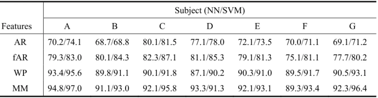
Experimental results of on-line performance are listed in Table 3.5. It can still be observed that WP and MM obtain higher recognition accuracy rate than RMS and DFA while MM is a little higher than WP (94.3% to 92.0%). However, the performance of NN is worse than that of SVM during on-line testing experiments (except subject D). The recognition accuracy rates of both of the two classifiers decrease compared with the performance during training period. The amplitude of decreasing for NN is larger than that of SVM.
Table 3.5. Performance of on-line testing. Subject (NN/SVM) Features A B C D E F G AR 70.2/74.1 68.7/68.8 80.1/81.5 77.1/78.0 72.1/73.5 70.0/71.1 69.1/71.2 fAR 79.3/83.0 80.1/84.3 82.3/87.1 81.1/85.3 79.1/81.3 75.1/81.1 77.7/80.2 WP 93.4/95.6 89.8/91.1 90.1/91.8 87.1/90.2 90.3/91.0 89.5/91.7 90.5/93.1 MM 94.8/97.0 91.1/93.0 92.1/95.8 93.3/91.3 92.1/93.1 89.3/93.4 92.3/96.4