Consistency properties of AIC, BIC, Cp and their
modifications in the growth curve model under a
large-(q, n) framework
Rie Enomoto, Tetsuro Sakurai and Yasunori Fujikoshi
(Received July 30, 2014; Revised October 2, 2014)Abstract. This paper is concerned with consistency properties of some criteria
for selecting row vectors of a k× p design matrix within individuals in the growth curve model, based on a sample of size n. Recently Enomoto, Sakurai and Fujikoshi (2013) showed that AIC and its modification have a consistency property for selecting hierarchical models of the row vectors under a condition on the order of the noncentrality matrix, assuming a large-(q, n) asymptotic framework such that q/n→ d ∈ [0, 1). We extend the result to a family of log-likelihood-based information criteria including AIC and BIC, and Cp. Further, their consistency properties are also obtained under a new condition on the order of the noncentrality matrix. Our results are checked numerically by conducting a Mote Carlo simulation.
AMS 2010 Mathematics Subject Classification. 62H12, 62H30.
Key words and phrases. AIC, BIC, Cp, Consistency property, Growth curve model, Large-(q, n) asymptotic framework, Simulation study.
§1. Introduction
The growth curve model introduced by Potthoff and Roy (1964) is written as
(1.1)
Y = AΘX +
E,
where Y; n
× p is an observation matrix, A; n × q is a design matrix across
individuals, X; k
× p is a design matrix within individuals, Θ is an unknown
matrix, and each row of
E is independent and identically distributed as a
p-dimensional normal distribution with mean 0 and an unknown covariance
matrix Σ. We assume that n
− p − k − 1 > 0, and rank(X) = k. If we consider
a polynomial regression of degree k
− 1 on the time t with q groups, then
(1.2)
A =
1
n10
· · ·
0
0
1
n2· · ·
0
..
.
..
.
. ..
..
.
0
0
· · · 1
nq
,
X =
1
1
· · ·
1
t
1t
2· · ·
t
p..
.
..
.
..
.
..
.
t
k1−1t
k2−1· · · t
kp−1
.
It is important to decide the degree in a polynomial growth curve model. In
general, we consider the problem of selecting the row vectors of X. Suppose
that j denotes a subset of ω =
{1, . . . , k} containing k
jelements, and X
jdenote the k
j× p matrix consisting of the rows of X indexed by the elements
of j. Note that X
ω= X and k
ω= k. We will let k
Adenote the number of
elements of a set A. We then consider the following candidate model M
jwith
k
jexplanatory variables defined by
(1.3)
M
j; Y = AΘ
jX
j+
E,
where Θ
jis a q
× k
jmatrix consisting of the columns of Θ indexed by the
elements of j, and
E has the same distribution as in (1.1). Here we note that
the design matrix A may be also an observation matrix of several explanatory
variables. For such an application, see Satoh and Yanagihara (2010). Let ˆ
Θ
jand ˆ
Σ
jbe the MLE’s of Θ
jand Σ under M
j, which are given by
ˆ
Θ
j= (A
′A)
−1A
′YS
−1X
′j(X
jS
−1X
′j)
−1,
ˆ
Σ
j=
1
n
(Y
− A ˆ
Θ
jX
j)
′(Y
− A ˆ
Θ
jX
j),
where S = (n
− q)
−1Y
′(I
n− PA
)Y, and P
A= A(A
′A)
−1A
′.
There are several criteria for selecting a “best” model from a family of
models M
j. The AIC and the BIC in our problem are given by
AIC = n log
| ˆ
Σ
j| + np(log 2π + 1) + 2
{
qk
j+
1
2
p(p + 1)
}
,
(1.4)
BIC = n log
| ˆ
Σ
j| + np(log 2π + 1) + (log n)
{
qk
j+
1
2
p(p + 1)
}
.
(1.5)
Here, the last term
{qk
j+p(p+1)/2
} is the number of independent parameters
under M
j. A consistent AIC (CAIC) based on Bozdogan (1987) is given by
(1.6)
CAIC = n log
| ˆ
Σ
j| + np(log 2π + 1) + (1 + log n)
{
qk
j+
1
2
p(p + 1)
}
.
We also consider the other modifications AICc, MAIC
Land MAIC
Hwhich are
given in Section 2. Further, we consider Cp defined by
and its modification MCp, which is given in Section 2.
In this paper, we assume that the true model is included in the full model
M
k. So, without loss of generality, we may assume that the minimum model
including the true model is expressed as M
j0for some j
0. Then, the true
model is expressed as expressed as
(1.8)
M
0: Y
∼ N
n×p(AΘ
0X
0, Σ
0⊗ I
n),
where Θ
0= Θ
j0, X
0= X
j0, and Σ
0is a given positive definite matrix. We
write k
0= k
j0. Let a set of candidate models denote by
F. The set of all
candidate models involves (2
k− 1) candidate models. A candidate model is
called an overspecified model or an underspecified model if it includes or does
not include the true model M
0. We denote a set of overspecified models and
a set of underspecified model by
F
+and
F
−, respectively.
In general, it can be seen that the criteria considered in this paper depend
through p, n, k
0, k and the characteristic roots of
(1.9)
Ω
j= Γ
′jΓ
j,
which is called a noncentrality matrix, where Γ
j= (A
′A)
1/2Θ
0X
0Σ
−1/20H
(j)2,
H
(j)1= (X
jΣ
−1/20)
′(X
jΣ
−10X
′j)
−1/2; p
× k
jand
(
H
(j)1, H
(j)2)
is an orthogonal
matrix.
It is known that AIC and Cp have not a consistency, but BIC and CAIC
have a consistency property, under a large-sample framework
(1.10)
p, q and k are fixed, n
→ ∞,
and Ω
j= O(n).
However, it is recently noted that AIC and Cp have a
consistency property in a high-dimensional framework. Such results can be
found in multivariate regression model, see, Fujikoshi, Sakurai and Yanagihara
(2014), Yanagihara, Wakaki and Fujikoshi (2014). Further, Enomoto, Sakurai
and Fujikoshi (2013) have noted that AIC and its modification MAIC
Hin our
problem have a consistency property for selecting hierarchical models of the
row vectors of X under a large-(q, n) framework such that
(1.11)
p and k are fixed, q
→ ∞, n → ∞, q/n → d ∈ [0, 1),
and Ω
j= O(n). In this paper we extend such properties to various criteria
including AIC, AICc, BIC, CAIC, MAIC
L, MAIC
H, Cp and MCp under Ω
j=
O(nq) as well as Ω
j= O(n).
When Ω
j= O(nq), it is noted that these
criteria have a consistency property, though some condition on the value of d
is imposed for AIC. When Ω
j= O(n), it is shown that BIC and CAIC have no
consistency property, but the other criteria have a consistency property under
some additional conditions. More precisely, we note that the probability of
selecting the true model by BIC or CAIC tends to zero. Our results are also
examined through a simulation experiment.
The present paper is organized as follows. In Section 2, we summarize
modifications of AIC and Cp. Consistency properties of a log-likelihood-based
information criterion are given in Section 3. In Section 4 we give consistency
properties of Cp and MCp. Numerical experiments are given in Section 5. In
Section 6, we summarize our conclusions. The proofs of our results are given
in Appendix.
§2. Modifications of AIC and Cp
In this section we summarize modifications of AIC and Cp, and review their
bias properties as estimators of the risks. As is well known, the AIC was
proposed as an approximately unbiased estimator of the risk defined by the
expected
−2×log-predictive likelihood. Let f(Y; Θ
j, Σ
j) be the density
func-tion of Y under M
j. Then the expected
−2×log-predictive likelihood under
M
jis defined by
(2.1)
R
A= E
∗YE
∗YF{
−2 log f(Y
F; ˆ
Θ
j, ˆ
Σ
j)
}
,
where ˆ
Σ
jand ˆ
Θ
jare the maximum likelihood estimators of Σ and Θ under
M
j, respectively. Here Y
F; n
× p may be regarded as a future random matrix
that has the same distribution as Y and is independent of Y, and E
∗denotes
the expectation with respect to the true model. The risk is expressed as
(2.2)
R
A= E
∗YE
∗YF{
−2 log f(Y; ˆ
Θ
j, ˆ
Σ
j)
}
+ b
A,
where
(2.3)
b
A= E
∗YE
∗YF{
−2 log f(Y
F; ˆ
Θ
j, ˆ
Σ
j) + 2 log f (Y; ˆ
Θ
j, ˆ
Σ
j)
}
.
The AIC and its modifications have been proposed by regarding the term
“
− b
A” as the bias term when we estimate R
Aby
−2 log f(Y; ˆ
Θ
j, ˆ
Σ
j) = n log
| ˆ
Σ
j| + np(log 2π + 1).
and considering an asymptotic approximation of b
A. A bias-corrected AIC is
defined by
where
b
A1=
− np +
n
2(p
− k
j)
n
− p + k
j− 1
+
n(n + q)(n
− q − 1)k
j(n
− q − p − 1)(n − q − p + k
j− 1)
.
(2.5)
Note that AICc is an exact unbiased estimator of R
Awhen M
jis an
overspec-ified model, i.e.
E(AICc) = R
A,
j
∈ F
+.
The term b
A1can be expressed as
b
A1= 2
{
qk
j+
1
2
p(p + 1)
}
+
(p
− k
j)(p
− k
j+ 1)
2n
− p + k
j− 1
+
k
j(2p + q
− k
j+ 1)(2q + p + 1)
n
− q − p − 1
(2.6)
+
(n + q)k
j(q + p
− k
j+ 1)(p
− k
j)
(n
− q − p − 1)(n − q − p + k
j− 1)
.
Therefore, we can easily see that under a large-sample framework
AICc = AIC + O(n
−1).
It is important that a modification has a small bias under underspecified
mod-els as well as overspecified modmod-els. Let b
A= b
A1+ b
A2. It is known (Enomoto,
Sakurai and Fujikoshi (2013)) that
b
A2=
−
n(p
− k
j)(p
− k
j+ 1)
n
− p + k
j− 1
+ 2(p
− k
j+ 1)ξ
1− ξ
2+ O
g(n
−1),
where O
g(n
i) denotes the term of i-th order with respect to n under (1.11),
ξ
1= tr
(
I
p−kj+
1
n
Ω
j)
−1,
ξ
2= ξ
12+ tr
(
I
p−kj+
1
n
Ω
j)
−2.
(2.7)
A modification under a large-sample framework (1.10) is given by
(2.8)
MAIC
L= n log
| ˆ
Σ
j| + np(log 2π + 1) + b
AL,
where
and
˜
ξ
1=
n
n
− q
{
tr(n ˆ
Σ
j)
−1(n
− q)S − k
j}
,
˜
ξ
2= ( ˜
ξ
1)
2+
(
n
n
− q
)
2[
tr
{(n ˆ
Σ
j)
−1(n
− q)S}
2− k
j]
.
Then, it is known (Satoh, Kobayashi and Fujikoshi (1997)) that under a
large-sample framework (1.10)
E (b
AL) =
{
b
A+ O(n
−2),
j
∈ F
+,
b
A+ O(n
−1),
j
∈ F
−.
The other modification based on a large-(n, q) framework (1.11) is given by
(2.10)
MAIC
H= n log
| ˆ
Σ
j| + np(log 2π + 1) + b
AH,
where
(2.11)
b
AH= b
A1+ ˆ
b
A2,
ˆ
b
A2= (p
− k
j+ 1)
{2ˆξ
1− (p − k
j)
} − ˆξ
2,
and ˆ
ξ
1= ˜
ξ
1,
ξ
ˆ
2= f ˜
ξ
2,
f =
3(n
− q)(p − k
j+ 1)(n
− 2p + 2k
j− 2)
n(n
− p + k
j− 1)
×
{
2(n
− q + 2)(p − k
j+ 2)
n + 2
+
(n
− q − 1)(p − k
j− 1)
n
− 1
}
−1.
Then, it is known (Enomoto, Sakurai and Fujikoshi (2013)) that under a
large-(n, q) framework (1.11)
E
(
ˆ
b
A)
=
{
b
A,
j
∈ F
+,
b
A+ O
g(n
−1),
j
∈ F
−.
The Cp in regression model was proposed by Mallows (1973) for the
uni-variate case. Sparks, Coutsourides and Troskie (1983) extended Mallows’
ap-proach to the multivariate case. Fujikoshi and Satoh (1997) gave a more
gen-eral approach to Cp in the multivariate case. The criterion in the growth curve
model may be essentially considered as an approximately unbiased estimator
of the risk of M
jdefined by
(2.12)
R
C= E
∗YE
∗YF{
trΣ
−10(Y
F− ˆY
j)
′(Y
F− ˆY
j)
}
where ˆ
Y
jis a predictor of Y under M
jgiven by ˆ
Y
j= X
jΘ
ˆ
j= P
jY, and Y
Fis the same random matrix as in (2.1). The risk is expressed as
(2.13)
R
C= E
∗Y{
(n
− k
j)tr ˆ
Σ
−1ωΣ
ˆ
j}
+ b
C,
where
(2.14)
b
C= E
∗YE
∗YF{
trΣ
−10(Y
F− ˆY
j)
′(Y
F− ˆY
j)
− (n − k
j)tr ˆ
Σ
−1 ωΣ
ˆ
j}
.
Similarly the Cp and its modification have been proposed by regarding “
−b
C”
as the bias term when we estimate R
Cby a minimum values of standardized
residuals sum of squares as
(n
− k
j)tr ˆ
Σ
−1 ωΣ
ˆ
j,
and by evaluating the bias term b
C. Satoh, Kobayashi and Fujikoshi (1997)
proposed the following Cp and its modification MCp:
Cp = ntr ˆ
Σ
jS
−1+ 2qk
j,
(2.15)
MCp = ntr ˆ
Σ
jS
−1+ q(p + k
j)
−
q(p
− k
j)(n
− q − k
j)
n
− q − p + k
j− 1
+
(
2k
j− p − 1
n
− q − p + k
j− 1
)
(2.16)
×
{
n(n
− q − p + k
j− 1)
n
− q
tr ˆ
Σ
jS
−1− (n − p + k
j− 1)p + qk
j}
.
The MCp satisfies
E(MCp) = R
C.
Further we can write MCp as
MCp =
{
1 +
2k
j− p + 1
n
− q
}
ntr ˆ
Σ
jS
−1+ 2qk
j+ p(p
− 2k
j+ 1)
= Cp + (2k
j− p + 1)
n
n
− q
tr ˆ
Σ
jS
−1+ p(p
− 2k
j+ 1).
(2.17)
§3. Consistency of a log-likelihood-based information criterion
We treat AIC and its modifications as a unified criterion
(3.1)
IC
j= n log det( ˆ
Σ
j) + np(log 2π + 1) + m
j,
which is called a log-likelihood-based information criterion, where m
jis a
positive constant expressing a penalty for the complexity of the model (1.3).
A specific criterion is given by specifying the individual penalty term m
j. It
contains AIC, BIC, CAIC, AICc, MAIC
Land MAIC
Has a special case, as
follows.
(3.2)
m
j=
2
{qk
j+ p(p + 1)/2
}
(AIC)
{qk
j+ p(p + 1)/2
} log n
(BIC)
{qk
j+ p(p + 1)/2
}(1 + log n) (CAIC)
b
A1,j(AICc)
b
AL,j(MAIC
L)
b
AH,j(MAIC
H)
.
Here the quantities b
A1,j, b
AL,jand b
AH,jare the same ones as in (2.6), (2.9)
and (2.11), respectively.
In this section we show that the asymptotic probability of selecting the
true model by AIC and its modifications goes to 1 when the number q and
the sample size n are approaching to
∞ as in (1.11), under some additional
assumptions. We denote the AIC for M
jby AIC
j. The best model chosen by
minimizing the AIC is written as
ˆ
j
AIC= arg min
j∈F
AIC
j,
which denotes the suffix j minimizing AIC
jwith respect to j
∈ F. Similar
notations are used for the other criteria. The consistency property of IC is
examined by using a key result (see, e.g., Fujikoshi, Enomoto and Sakurai
(2013))
(3.3)
|(n − q)S|
|n ˆ
Σ
j|
=
|W
(j)|
|W
(j)+ B
(j)|
,
where W
(j)are independently distributed as a Wishart distribution W
p−kj(n
−
q, I
p−kj) and a noncentral distribution W
p−kj(q, I
p−kj; Ω
j), respectively. The
matrix Ω
jis defined by (1.9).
Our main assumptions are summarized as follows:
A1 (The true model M
0): j
0∈ F.
A2 (The asymptotic framework): q
→ ∞, n → ∞, q/n → d ∈ [0, 1).
A3 (The order assumption (i) of Ω
j): For j
∈ F
−,
Ω
j= n∆
j= O
g(n) and
lim
q/n→d
∆
j= ∆
∗ j.
A4 (The order assumption (ii) of Ω
j): For j
∈ F
−,
Ω
j= nqΞ
j= O
g(nq) and
lim
q/n→d
Ξ
j= Ξ
∗ j.
Our consistency properties of a log-likelihood-based information criterion are
given in two theorems, depending on the assumptions A3 and A4 on the order
of the noncentrality matrix Ω
jas follows.
Theorem 3.1. Suppose that the assumptions A1, A2 and A3 are satisfied.
(1) Let d
a(
≈ 0.797) be the constant satisfying log(1−d
a)+2d
a= 0. Further,
assume that d
∈ [0, d
a), and
A5: For any j
∈ F
−,
log
|I
p−kj+ ∆
∗
j
| > (k
0− k
j)
{2d + log(1 − d)}.
Then, the model selection criterion AIC is consistent, i.e., the asymptotic
probability of selecting the true model j
0by the AIC tends to 1, which may be
stated as
lim
q/n→d
P (ˆ
j
AIC= j
0) = 1.
(2) Suppose that
A6: For any j
∈ F
−,
log
|I
p−kj+ ∆
∗ j| > (k
0− k
j)
{
2d
1
− d
+ log(1
− d)
}
.
Then, the model selection criteria AICc, MAIC
Land MAIC
Hare consistent.
(3) The model selection criteria BIC and CAIC are not consistent. More
precisely, the probability of selecting the true model by BIC or CAIC tends to
zero.
Theorem 3.1 is an extension of Enomoto, Sakurai and Fujikoshi (2013)
which proves consistency of AIC and MAIC
Hin the case of selection of
hier-arichical models on the row vectors of X.
Theorem 3.2. Suppose that the assumptions A1, A2 and A4 are satisfied.
(1) If d
∈ [0, d
a), then, the model selection criterion AIC is consistent. Here
d
ais given Theorem 3.1.
(2) Suppose that for any j
∈ F
−,
|Ξ
j| > 0. Then, the model selection
criteria AICc, BIC, CAIC, MAIC
Land MAIC
Hare consistent.
§4. Consistency of Cp and MCp
In this section we give consistency properties of Cp and MCp. The derivation
is done in a way similar to one for a log-likelihood-based information criterion,
with the help of
n
n
− q
tr ˆ
Σ
jS
−1= tr(n ˆ
Σ
j)
{(n − q)S}
−1= p + trB
(j)W
−1(j),
(4.1)
where W
(j)and B
(j)are the same random matrices as in (3.3).
Theorem 4.3. Suppose that the assumptions A1, A2 and A3 are satisfied.
Further, assume that
A7: For any j
∈ F
−,
tr∆
∗j> d(k
0− k
j).
Then, the model selection criteria Cp and MCp are consistent.
Theorem 4.4. Suppose that the assumptions A1, A2 and A4 are satisfied.
Further, suppose that for any j
∈ F
−, trΞ
∗j> 0. Then, the model selection
criteria Cp and MCp are consistent.
These results will be worthy of note, since Cp and MCp are known to be
inconsistent under a large-sample framework.
§5. Simulation study
In this section, we numerically examine the validity of our claims and the speed
of the convergences of the criteria. Monte Carlo simulations were considered
for several different values of n and q = dn, where p = 5, n = 50, 100, 200,
n
1=
· · · = n
q= n/q and d = 0.1, 0.2. We constructed a 5
× 5 matrix X
as in (1.2) of explanatory variables with t
i= 1 + (i
− 1)(p − 1)
−1. The true
covariance matrix Σ
0was determined such that its (i, j)th element is ρ
|i−j|,
where ρ = 0.2, 0.8. We consider the five candidate models M
1, . . . , M
5, where
M
jdenotes the model with the first j rows of X. So, in this section a subset
j means j =
{1, . . . , j}. We assume that M
2is the minimum model including
the true model. The true model are included in M
2, M
3, M
4, M
5, but it is not
included in M
1. Therefore, Ω
j=
0
when M
2, M
3, M
4, M
5, and Ω
j̸=
0
when
M
1.
5.1.
The case of order assumption (i)
As a realization of Ω
j= O
g(n) we assume that Θ
0= 1
q1
′2. Then, the
non-centrality matrix Ω
jis expressed as
Ω
j= H
(j)2 ′Σ
−1/20 ′X
′0Θ
′0A
′AΘ
0X
0Σ
−1/20H
(j)2= H
(j)2 ′Σ
−1/20 ′X
′01
21
′q
n
10
· · ·
0
0
n
2· · ·
0
..
.
..
.
. .. ...
0
0
· · · n
q
1
q1
′2X
0Σ
−1/20H
(j)2= H
(j)2 ′Σ
−1/20 ′X
′0(
n
n
n
n
)
X
0Σ
−1/20H
(j)2.
Further, X
0, Σ
−1/20and H
(j)2do not depend on n and q. Therefore, Ω
j=
O
g(n). Moreover, the convergent values in A5, A6 and A7 for consistency are
calculated as follows:
ρ d log|Ip−kj + ∆ ∗ j| 2d + log(1 − d) 2d/(1 − d) + log(1 − d) tr∆∗j 0.2 0.1 0.440 0.095 0.117 0.552 0.2 0.440 0.177 0.277 0.552 0.8 0.1 0.614 0.095 0.117 0.847 0.2 0.614 0.177 0.277 0.847Here,F− contains a subset{1} only. Therefore, we can see that in our setting the assumptions A5, A6 and A7 are satisfied.
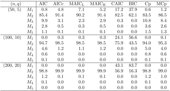
The selection probabilities (%) based on Monte Carlo simulations with 104
itera-tions are summarized in Tables 1∼ 4. From these tables we can point the following tendencies.
• We can see that CAIC and BIC have no consistency property. In general, they
chose M1 with high probabilities, though they have a tendency of choosing M2
for d = 0.1 and ρ = 0.8.
• MAICHchooses M2more frequently than MAICL. Similarly, MCp chooses M2
more frequently than Cp.
• As q increases under n being fixed, AIC, Cp and MCp choose M2 more
fre-quently, but the other criteria choose M2more fewer.
• For the speed of convergences to 1, the case ρ = 0.8 is faster than the case ρ = 0.2.
• AIC, Cp and MCp have a tendency of choosing overspecified models than AICc,
MAICL and MAICH.
• AICc, MAICL and MAICHhave a tendency of choosing underspecif ied modes
• When d = 0.2 and n and q are small, AIC chooses the true model more
fre-quently than AICc, MAICL and MAICH.
• MCp chooses the true model more frequently than Cp in all the cases except
Table 1. Selection probabilities (%) for d = 0.1 and ρ = 0.2.
(n, q) AIC AICc MAICL MAICH CAIC BIC Cp MCp
(50, 5) M1 0.8 4.8 7.1 5.2 17.2 37.9 0.6 1.2 M2 85.4 91.4 90.2 91.4 82.5 62.1 83.5 86.5 M3 9.9 3.1 2.3 2.9 0.3 0.0 10.8 8.4 M4 2.8 0.5 0.3 0.5 0.0 0.0 3.6 2.6 M5 1.1 0.1 0.1 0.1 0.0 0.0 1.5 1.3 (100, 10) M1 0.0 0.3 0.3 0.3 24.1 56.6 0.0 0.1 M2 94.7 98.5 98.5 98.5 75.9 43.5 94.0 95.3 M3 4.6 1.2 1.1 1.2 0.0 0.0 5.0 4.0 M4 0.6 0.0 0.0 0.0 0.0 0.0 0.8 0.6 M5 0.1 0.0 0.0 0.0 0.0 0.0 0.1 0.1 (200, 20) M1 0.0 0.0 0.0 0.0 43.1 83.7 0.0 0.0 M2 98.8 99.9 99.9 99.9 56.9 16.3 98.8 99.0 M3 1.2 0.1 0.1 0.1 0.0 0.0 1.2 1.0 M4 0.1 0.0 0.0 0.0 0.0 0.0 0.1 0.0 M5 0.0 0.0 0.0 0.0 0.0 0.0 0.0 0.0
Table 2. Selection probabilities (%) for d = 0.2 and ρ = 0.2.
(n, q) AIC AICc MAICL MAICH CAIC BIC Cp MCp
(50, 10) M1 5.5 49.4 55.5 52.0 70.1 92.0 4.2 9.6 M2 85.6 50.4 44.4 47.9 29.9 8.0 85.0 83.4 M3 7.2 0.2 0.1 0.2 0.0 0.0 8.4 5.5 M4 1.4 0.0 0.0 0.0 0.0 0.0 1.9 1.2 M5 0.4 0.0 0.0 0.0 0.0 0.0 0.6 0.4 (100, 20) M1 0.9 22.9 24.9 23.8 95.9 99.9 0.8 1.7 M2 96.6 77.1 75.1 76.2 4.1 0.1 96.6 96.5 M3 2.4 0.0 0.0 0.0 0.0 0.0 2.5 1.7 M4 0.1 0.0 0.0 0.0 0.0 0.0 0.2 0.1 M5 0.0 0.0 0.0 0.0 0.0 0.0 0.0 0.0 (200, 40) M1 0.0 7.0 7.4 7.1 100.0 100.0 0.0 0.1 M2 99.7 93.0 92.7 92.9 0.0 0.0 99.7 99.7 M3 0.3 0.0 0.0 0.0 0.0 0.0 0.3 0.2 M4 0.0 0.0 0.0 0.0 0.0 0.0 0.0 0.0 M5 0.0 0.0 0.0 0.0 0.0 0.0 0.0 0.0
Table 3. Selection probabilities (%) for d = 0.1 and ρ = 0.8.
(n, q) AIC AICc MAICL MAICH CAIC BIC Cp MCp
(50, 5) M1 0.0 0.3 0.5 0.3 2.2 9.1 0.0 0.0 M2 85.9 96.2 96.8 96.4 97.4 90.9 83.8 87.6 M3 10.1 3.0 2.3 2.8 0.3 0.0 11.1 8.5 M4 3.0 0.5 0.3 0.5 0.0 0.0 3.7 2.7 M5 1.0 0.1 0.1 0.1 0.0 0.0 1.4 1.2 (100, 10) M1 0.0 0.0 0.0 0.0 1.5 10.3 0.0 0.0 M2 94.9 98.6 98.7 98.7 98.5 89.7 94.4 95.5 M3 4.4 1.3 1.2 1.3 0.0 0.0 4.8 3.8 M4 0.6 0.1 0.0 0.1 0.0 0.0 0.7 0.5 M5 0.1 0.0 0.0 0.0 0.0 0.0 0.2 0.1 (200, 20) M1 0.0 0.0 0.0 0.0 1.5 15.7 0.0 0.0 M2 98.9 99.9 99.9 99.9 98.6 84.3 98.7 99.0 M3 1.1 0.1 0.1 0.1 0.0 0.0 1.2 1.0 M4 0.1 0.0 0.0 0.0 0.0 0.0 0.1 0.1 M5 0.0 0.0 0.0 0.0 0.0 0.0 0.0 0.0
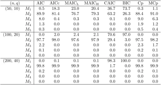
Table 4. Selection probabilities (%) for d = 0.2 and ρ = 0.8.
(n, q) AIC AICc MAICL MAICH CAIC BIC Cp MCp
(50, 10) M1 0.5 18.3 23.0 20.4 36.7 73.7 0.3 1.1 M2 89.9 81.4 76.7 79.3 63.2 26.3 88.4 91.0 M3 8.0 0.4 0.3 0.3 0.1 0.0 9.0 6.3 M4 1.3 0.0 0.0 0.0 0.0 0.0 1.9 1.2 M5 0.3 0.0 0.0 0.0 0.0 0.0 0.5 0.4 (100, 20) M1 0.0 2.0 2.4 2.1 70.6 97.0 0.0 0.0 M2 97.7 98.0 97.6 97.9 29.4 3.0 97.5 98.2 M3 2.2 0.0 0.0 0.0 0.0 0.0 2.3 1.7 M4 0.1 0.0 0.0 0.0 0.0 0.0 0.2 0.1 M5 0.0 0.0 0.0 0.0 0.0 0.0 0.0 0.0 (200, 40) M1 0.0 0.1 0.1 0.1 98.3 100.0 0.0 0.0 M2 99.8 99.9 99.9 99.9 1.7 0.0 99.8 99.9 M3 0.2 0.0 0.0 0.0 0.0 0.0 0.2 0.1 M4 0.0 0.0 0.0 0.0 0.0 0.0 0.0 0.0 M5 0.0 0.0 0.0 0.0 0.0 0.0 0.0 0.0
5.2. The case of order assumption (ii)
As a realization of Ωj = Og(nq) we assume that Θ0 =√q1q1′2. Then, the
noncen-trality matrix Ωj is expressed as
Ωj= H (j) 2 ′ Σ−1/20 ′X′0Θ′0A′AΘ0X0Σ−1/20 H (j) 2 = qH(j)2 ′Σ−1/20 ′X′0121′q n1 0 · · · 0 0 n2 · · · 0 .. . ... . .. ... 0 0 · · · nq 1q1′2X0Σ−1/20 H (j) 2 = H(j)2 ′Σ−1/20 ′X′0 ( nq nq nq nq ) X0Σ−1/20 H (j) 2 .
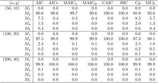
Therefore, Ωj= Og(nq). The selection probabilities (%) are summarized in Tables 5 ∼ 8. From these tables we can point the following tendencies.
• We can see that all the eight criteria have consistency property.
• MAICHand MCp choose the true model more frequently than MAICLand Cp,
respectively.
• As q increases under n being fixed, all the criteria choose the true model more
frequently.
• In general, AIC, Cp and MCp have a tendency of choosing larger models when n and q are small.
• It seems that all the criteria doe not choose underspecified models.
• For the speed of convergence to the true model, BIC and CAIC are more faster
Table 5. Selection probabilities (%) for d = 0.1 and ρ = 0.2.
(n, q) AIC AICc MAICL MAICH CAIC BIC Cp MCp
(50, 5) M1 0.0 0.0 0.0 0.0 0.0 0.0 0.0 0.0 M2 86.1 96.0 96.9 96.3 99.6 99.9 84.2 87.5 M3 9.9 3.3 2.6 3.1 0.4 0.1 10.8 8.6 M4 3.0 0.5 0.4 0.5 0.0 0.0 3.6 2.6 M5 1.0 0.1 0.1 0.1 0.0 0.0 1.5 1.2 (100, 10) M1 0.0 0.0 0.0 0.0 0.0 0.0 0.0 0.0 M2 95.2 98.7 98.8 98.8 100.0 100.0 94.6 95.7 M3 4.2 1.2 1.1 1.2 0.0 0.0 4.6 3.6 M4 0.6 0.1 0.1 0.1 0.0 0.0 0.8 0.6 M5 0.0 0.0 0.0 0.0 0.0 0.0 0.1 0.0 (200, 20) M1 0.0 0.0 0.0 0.0 0.0 0.0 0.0 0.0 M2 98.8 99.8 99.8 99.8 100.0 100.0 98.8 99.0 M3 1.1 0.2 0.2 0.2 0.0 0.0 1.2 1.0 M4 0.0 0.0 0.0 0.0 0.0 0.0 0.0 0.0 M5 0.0 0.0 0.0 0.0 0.0 0.0 0.0 0.0
Table 6. Selection probabilities (%) for d = 0.2 and ρ = 0.2.
(n, q) AIC AICc MAICL MAICH CAIC BIC Cp MCp
(50, 10) M1 0.0 0.0 0.0 0.0 0.0 0.0 0.0 0.0 M2 90.4 99.5 99.6 99.6 99.9 100.0 88.8 92.2 M3 7.7 0.5 0.4 0.4 0.1 0.0 8.7 6.0 M4 1.5 0.0 0.0 0.0 0.0 0.0 1.9 1.3 M5 0.4 0.0 0.0 0.0 0.0 0.0 0.6 0.5 (100, 20) M1 0.0 0.0 0.0 0.0 0.0 0.0 0.0 0.0 M2 97.4 100.0 100.0 100.0 100.0 100.0 97.3 98.1 M3 2.4 0.0 0.0 0.0 0.0 0.0 2.5 1.7 M4 0.2 0.0 0.0 0.0 0.0 0.0 0.2 0.2 M5 0.0 0.0 0.0 0.0 0.0 0.0 0.0 0.0 (200, 40) M1 0.0 0.0 0.0 0.0 0.0 0.0 0.0 0.0 M2 99.9 100.0 100.0 100.0 100.0 100.0 99.9 99.9 M3 0.1 0.0 0.0 0.0 0.0 0.0 0.2 0.1 M4 0.0 0.0 0.0 0.0 0.0 0.0 0.0 0.0 M5 0.0 0.0 0.0 0.0 0.0 0.0 0.0 0.0
Table 7. Selection probabilities (%) for d = 0.1 and ρ = 0.8.
(n, q) AIC AICc MAICL MAICH CAIC BIC Cp MCp
(50, 5) M1 0.0 0.0 0.0 0.0 0.0 0.0 0.0 0.0 M2 86.9 96.5 97.3 96.7 99.7 100.0 84.6 88.3 M3 9.3 2.9 2.3 2.8 0.3 0.0 10.6 8.1 M4 2.8 0.4 0.3 0.4 0.0 0.0 3.5 2.6 M5 1.0 0.1 0.1 0.1 0.0 0.0 1.3 1.1 (100, 10) M1 0.0 0.0 0.0 0.0 0.0 0.0 0.0 0.0 M2 94.3 98.6 98.9 98.7 100.0 100.0 93.4 94.8 M3 4.9 1.3 1.1 1.3 0.0 0.0 5.5 4.4 M4 0.8 0.1 0.1 0.1 0.0 0.0 1.0 0.7 M5 0.1 0.0 0.0 0.0 0.0 0.0 0.1 0.1 (200, 20) M1 0.0 0.0 0.0 0.0 0.0 0.0 0.0 0.0 M2 98.9 99.8 99.8 99.8 100.0 100.0 98.9 99.1 M3 1.0 0.2 0.2 0.2 0.0 0.0 1.1 0.8 M4 0.0 0.0 0.0 0.0 0.0 0.0 0.0 0.0 M5 0.0 0.0 0.0 0.0 0.0 0.0 0.0 0.0
Table 8. Selection probabilities (%) for d = 0.2 and ρ = 0.8.
(n, q) AIC AICc MAICL MAICH CAIC BIC Cp MCp
(50, 10) M1 0.0 0.0 0.0 0.0 0.0 0.0 0.0 0.0 M2 90.6 99.6 99.7 99.6 100.0 100.0 88.9 92.6 M3 7.5 0.4 0.3 0.4 0.0 0.0 8.5 5.7 M4 1.5 0.0 0.0 0.0 0.0 0.0 2.0 1.3 M5 0.4 0.0 0.0 0.0 0.0 0.0 0.6 0.4 (100, 20) M1 0.0 0.0 0.0 0.0 0.0 0.0 0.0 0.0 M2 97.5 99.9 99.9 99.9 100.0 100.0 97.3 98.1 M3 2.3 0.1 0.1 0.1 0.0 0.0 2.5 1.8 M4 0.2 0.0 0.0 0.0 0.0 0.0 0.2 0.1 M5 0.0 0.0 0.0 0.0 0.0 0.0 0.1 0.0 (200, 40) M1 0.0 0.0 0.0 0.0 0.0 0.0 0.0 0.0 M2 99.9 100.0 100.0 100.0 100.0 100.0 99.9 99.9 M3 0.1 0.0 0.0 0.0 0.0 0.0 0.1 0.1 M4 0.0 0.0 0.0 0.0 0.0 0.0 0.0 0.0 M5 0.0 0.0 0.0 0.0 0.0 0.0 0.0 0.0 §6. Concluding remarks
This paper discusses with consistency properties of a log-likelihood criterion including AIC and its modifications, Cp and its modification MCp for selecting the row vectors of a design matrix X within individuals in the growth curve model (1.1) under a large-(q, n) framework (1.11). The log-likelihood criterion includes AIC, AICc, BIC, CAIC, MAICL and MAICH as a special case. The consistency properties depend
on the order of the noncentrality matrix Ωj of model Mj. When Ωj = Og(n), it
is noted that AIC, AICc, MAICL and MAICH, Cp and MCp are consistent under
some additional assumptions on Ωj. However, BIC and CAIC are not consistent, and
more precisely, the probability of selecting the true model by BIC or CAIC tends to zero. When Ωj = Og(nq), it is noted that these criteria have a consistency property,
though some condition on the value of d is imposed for AIC.
In a traditional growth curve model it is assumed that the dimension p is not large or moderate. However, it is also important to analyze the data such that p is large. Further, the number k of explanatory variables within individuals will be large. This suggests to study asymptotic properties of these model selection criteria under a high-dimensional framework such that
k → ∞, p → ∞, q → ∞, n → ∞,
k/n→ b ∈ [0, 1), p/n → c ∈ [0, 1), q/n → d ∈ [0, 1),
(6.1)
where 1 > c≥ d ≥ 0. Modifications of AIC and Cp and their consistency properties under (6.1) should be also studied. These works are left as a future subject.
§7. Appendix: Proofs of Theorems
First we explain an outline of our proof. In general, letF be a finite set of candidate models j (or Mj). Assume that j0is the minimum model including the true model and j0∈ F. Let Tj(n) be a general criterion for model j, which depends on a parameter n.
The best model chosen by minimizing Tj(n) is written as ˆjT(n) = arg minj∈FTj(n).
Suppose that we are interested in asymptotic behavior of ˆjT(n) when n tends to∞.
In order to show a consistency of Tj(n), we may check a sufficient condition such that
for any j̸= j0∈ F, there exists a sequence {an} with an> 0, an{Tj(n)− Tj0(n)}
p
→ bj > 0.
In fact, the condition implies that for any j̸= j0∈ F,
P (ˆjT(n) = j)≤ P (Tj(n) < Tj0(n))→ 0, and P (ˆjT(n) = j0) = 1− ∑ j̸=j0∈F P (ˆjT(n) = j)→ 1.
On the other hand, relating to showing an inconsistency of ˆjT(n), assume that for
some j̸= j0∈ F and for a sequence {an} with an> 0, an{Tj(n)− Tj0} p → dj< 0. Then we have P (Tj(n) < Tj0(n))→ 1. Further, we have P (ˆjT(n) = j0)≤ P (Tj0(n) < Tj(n)) = 1− P (Tj(n) < Tj0(n))→ 0.
This means that ˆjT(n) is inconsistent, and further the probability of selecting the
true model tends to zero.
Proof of Theorem 3.1
The consistency properties of AIC and MAICH have been essentially proved by
Enomoto, Sakurai and Fujikoshi (2013) who proved for the case of selecting hierar-chical models of the row vectors of X. The following result was used there:
log| ˆΣj| − log | ˆΣj0| = log |n ˆΣj| − log |n ˆΣj0|
=− log|(n − q)S| |n ˆΣj| + log|(n − q)S| |n ˆΣj0| =− log |W(j)| |W(j)+ B(j)| + log |W(j0)| |W(j0)+ B(j0)| .
Further, noting that 1 nW(j) p → (1 − d)Ip−kj, and 1 nB(j) p → dIp−kj + ∆ ∗ j,
the following result was used:
− log |W(j)| |W(j)+ B(j)| p → log |Ip−kj+ ∆ ∗ j| − (p − kj) log(1− d).
These imply that 1 n(ICj− ICj0)− 1 n(mj− mj0) p → log |Ip−kj + ∆ ∗ j| + (kj− k0) log(1− d), (7.1)
since ∆j0=
0
. For the penalty terms, it is easily seen that(7.2) 1 n(mj− mj0) p → { 2d(kj− k0) (AIC) 2d(1− d)−1(kj− k0) (AICc) , and (7.3) 1 n log n(mj− mj0) p → (kj− k0)d (BIC, CAIC).
Now we shall prove the case of AICc. From (7.1) and (7.2) we have 1 n(AICcj− AICcj0) p → log |Ip−kj+ ∆ ∗ j| + (kj− k0) { 2d 1− d+ log(1− d) } . (7.4)
Therefore, when j∈ F+, log|Ip−kj + ∆ ∗
j| = 0, and hence
since (2d)/(1− d) + log(1 − d) is always positive. When j ∈ F−, we have AICcj−
AICcj0> 0 from (7.4) and the assumption A6. These imply the consistency of AICc.
For the case d = 0, we need to modify the above proof slightly. For example, we can prove by considering the limit of (1/q)(AICcj− AICcj0) in stead of (1/n)(AICcj−
AICcj0). In the following, we give a proof for 0 < d < 1, and the proof of d = 0 is
omitted.
For the case of BIC, from (7.1) and (7.3) we have 1
n log n(BICj− BICj0)
p
→ (kj− k0)d.
This implies that for some j such that j ∈ F− and kj− k0 < 0, BICj < BICj0 for
large n. These show an inconsistency of BIC and
P (ˆjBIC= j0)→ 0.
The case of CAIC is proved similarly as the one of BIC.
In order to prove the case of MAICL, it needs to examine asymptotic behavior of
˜bA2as in Enomoto, Sakurai and Fujikoshi (2013), which gives an asymptotic behavior of ˆbA2. We can express tr(n ˆΣj)−1(n− q)S = j + trQj, tr { (n ˆΣj)−1(n− q)S }2 = j + trQ2j, where Qj= W(j)(W(j)+ B(j))−1. Using Qj p → (1 − d)(Ip−kj + ∆ ∗ j )−1 , we have ˜ ξ1 p → ξ10= tr(I + ∆∗j)−1, ˜ ξ2 p → ξ20= { tr(I + ∆∗j)−1}2+ tr(I + ∆∗j)−2.
From these results we have (1/n)˜bA2→ 0. Therefore, we get that the consistency of
MAICL is the same as the one of AICc.
Proof of Theorem 3.2
First we note that when j∈ F+, from (7.1) we have
(7.5) 1 n(ICj− ICj0)− 1 n(mj− mj0) p → (kj− k0) log(1− d), j∈ F+.
On the other hand, when j∈ F−, 1 nW(j) p → (1 − d)Ip−kj, 1 nqB(j) p → Ξj, and hence
log| ˆΣj| − log | ˆΣj0| = − log
|W(j)| |W(j)+ B(j)| + log |W(j0)| |W(j0)+ B(j0)| =− log | 1 nW(j)| | 1 nq(W(j)+ B(j))|q p−kj + log |W(j0)| |W(j0)+ B(j0)| .
These imply that (7.6) 1 n log q(ICj− ICj0)− 1 n log q(mj− mj0) p → p − kj, j∈ F−.
Using (7.5) and (7.6) we can prove Theorem 3.2 by the same line as in Theorem 3.1. Its detail is omitted.
Proofs of Theorems 4.3 and 4.4
Noting that n n− qtr ˆΣjS −1 = tr(n ˆΣ j){(n − q)S}−1 = p + trB(j)W−1(j), we have 1 n− q(Cpj− Cpj0) = trB(j)W −1 (j)− trB(j0)W −1 (j0)+ 2q n− q(kj− k0).
First consider the case Ωj = Og(n) = n∆j. In this case
trB(j)W−1(j) p → 1 1− d ( dIp−kj + ∆ ∗ j ) .
When j∈ F+, ∆j=
0
, and hence1 n− q ( Cpj− Cpj0)→p d 1− d(p− kj)− d 1− d(p− k0) + 2d 1− d(kj− k0) = (kj− k0)· d 1− d. When j∈ F−, 1 n− q ( Cpj− Cpj 0 ) p →(kj− k0)· d 1− d+ 1 1− dtr∆ ∗ j = 1 1− d{tr∆ ∗ j+ d(kj− k0)}.
Therefore, if tr∆∗j > d(k0− kj), j∈ F−, then Cp is consistent.
Next we consider the case Ωj= Og(nq) = nqΞj. When j ∈ F+, the result in the
case Ωj= Og(n), we have that{1/(n − q)}
(
Cpj− Cpj
0
)
> 0. When j∈ F−, we can see that for j∈ F−
1 q(n− q){Cpj− Cpj0} p → 1 1− dtrΞ ∗ j.
This implies Theorem 4.4 in the case Cp.
Finally we show that the above consistency properties of Cp hold for MCp. We have seen that when Ωj= Og(n),
n n− q ( tr ˆΣjS−1− tr ˆΣj0S −1)= trB (j)W−1(j)− trB(j0)W −1 (j0) p → 1 1− d{tr∆ ∗ j− d(kj− k0)}.
When Ωj= Og(nq), we have seen that n q(n− q) ( tr ˆΣjS−1− tr ˆΣj0S −1)= 1 q ( trB(j)W−1(j)− trB(j0)W −1 (j0) ) p → 1 1− dtrΞ ∗ j.
Using these results and a relationship between Cp and MCp given in (2.17), we have that MCp has the same consistency properties as the ones of Cp.
Acknowledgement
The first author’s research was in part supported by Grant-in-Aid for Research Activ-ity Start-up 25880017. The third author’s research was in part supported by Grant-in-Aid for Scientific Research (C) 25330038.
References
[1] Bozdogan, H. (1987). Model selection and Akaike’s information criterion (AIC): the general theory and its analytical extensions. Psychometrika, 52, 345–370.
[2] Enomoto, R., Sakurai, T. and Fujikoshi, Y. (2013). Consistency of AIC and its modification in the growth curve model under a large-(q, n) framework.
SUT J. Math. . 49, 93–107.
[3] Fujikoshi, Y. and Satoh, K. (1997). Modified AIC and Cpin multivariate
linear regression. Biometrika, 84, 707–716.
[4] Fujikoshi, Y., Enomoto, R. and Sakurai, T. (2013). High-dimensional AIC in the growth curve model. J. Multivariate Anal., 122, 239–250. [5] Fujikoshi, Y., Sakurai, T. and Yanagihara, H. (2014). Consistency of
high-dimensional AIC-type and Cp-type criteria in multivariate linear
regres-sion. J. Multivariate Anal., 123, 184–200.
[6] Mallows, C. L. (1973). Some comments on Cp. Technometrics, 15, 661–675.
[7] Potthoff, R. F. and Roy, S. N. (1964). A generalized multivariate analysis of variance model useful especially for growth curve problems. Biometrika,
51, 313–326.
[8] Satoh, K. and Yanagihara, H. (2010). Estimation of varying coefficients for a growth curve model. Amer. J. Math. Management Sci., 30, 243–256. [9] Satoh, K., Kobayashi, M. and Fujikoshi, Y. (1997). Variable selection for
the growth curve model. J. Multivariate Anal., 60, 277–292.
[10] Sparks, R. S., Coutsourides, D. and Troskie, L. (1983). The multivariate
[11] Yanagihara, H., Wakaki, H. and Fujikoshi, Y. (2014). A consistency property of AIC for multivariate linear model when the dimension and the sample size are large. Submitted for publication.
Rie Enomoto
Department of Mathematical Information Science, Tokyo University of Science 1-3 Kagurazaka, Shinjuku-ku, Tokyo 162-8601, Japan
E-mail : [email protected]
Tetsuro Sakurai
Center of General Education, Tokyo University of Science, Suwa 5000-1 Toyohira, Chino, Nagano 391-0292, Japan
Yasunori Fujikoshi
Department of Mathematics, Graduate School of Science, Hiroshima University 1-3-1 Kagamiyama, Higashi-Hiroshima, Hiroshima, 739-8626, Japan