Decomposition of diamond model for square
contingency tables with ordered categories
Kiyotaka Iki
(Received March 13, 2018; Revised June 8, 2018)
Abstract. For square contingency tables with the same row and column ordinal classifications, this paper shows that the diamond model holds if and only if the weighted covariance for the difference between the row and column classifications and the sum of them equals zero and the uniform association diamond model holds. An example is given.
AMS 2010 Mathematics Subject Classification. 62H17.
Key words and phrases. Decomposition, diamond model, odds ratio, uniform
association, weighted covariance.
§1. Introduction
Consider an R× R square contingency table with the same row and column ordinal classifications. Let X and Y denote the row and column variables, respectively, and let pij denote the probability that an observation will fall in (i, j)th cell of the table (i = 1, . . . , R; j = 1, . . . , R). The independence model is defined by
pij = µαiβj for i = 1, . . . , R; j = 1, . . . , R.
Goodman (1979) refereed to this model as the null association model. The uniform association model is defined by
pij = µαiβjθij for i = 1, . . . , R; j = 1, . . . , R;
see Goodman (1979, 1981) and Agresti (1984, p.78). A special case of this model with θ = 1 is the independence model. If the independence model holds, then the covariance between X and Y equals zero; but the converse does not hold. Tomizawa, Miyamoto and Sakurai (2008) gave the theorem
that the independence model holds if and only if the covariance between X and Y equals zero and the uniform association model holds.
The diamond (DD) model (Goodman, 1985) is defined by
pij = µδi−jγi+j for i = 1, . . . , R; j = 1, . . . , R.
As described by Goodman (1985), the DD model states that there is null association between the difference-diagonal classification (i.e., the difference between the row and column classification) and the sum-diagonal classification (i.e., the sum of the row and column classification). Consider the (2R − 1)× (2R − 1) table of the diamond shape formed by rotating to the original
R× R table forty-five degrees so that the 2R − 1 difference-diagonals in the
original table form the entries in the rows of the diamond, and corresponding 2R− 1 sum-diagonals in the original table form the entries in the columns of the diamond. Let S∗ denote a set of cells of the diamond shape in the (2R− 1) × (2R − 1) table. Thus,
S∗={(s, t)|s = i − j, t = i + j; i = 1, . . . , R; j = 1, . . . , R}.
Let p∗stdenote the corresponding probability for row value s and column value
t for (s, t)∈ S∗, in the (2R− 1) × (2R − 1) table, i.e.,
p∗st = ps+t
2 ,
t−s
2 for (s, t)∈ S ∗.
Let θ∗(k<l;s<t) denote the odds ratio for row values k and l and column values
s and t in the (2R− 1) × (2R − 1) table of the diamond shape. Thus, θ(k<l;s<t)∗ = p
∗ ksp∗lt
p∗ktp∗ls for (k, s), (k, t), (l, s), (l, t)∈ S
∗.
Then, the DD model is also expressed as
θ∗(k<l;s<t)= 1 for (k, s), (k, t), (l, s), (l, t)∈ S∗.
For the original R×R table, the uniform association diamond (UADD) model is defined by
pij = µδi−jγi+jϕ(i−j)(i+j) for i = 1, . . . , R; j = 1, . . . , R;
see Tomizawa (1994). A special case of this model with ϕ = 1 is the DD model. Using the odds-ratios defined for the (2R− 1) × (2R − 1) table of the diamond shape, the UADD model is also expressed as
Thus, the UADD model is uniform association model in (2R− 1) × (2R − 1) table of the diamond shape. If the DD model holds, then the UADD model holds; but the converse does not hold. Therefore, for the (2R− 1) × (2R − 1) table of the diamond shape, we are interested in what covariance structure between the difference-diagonal classification and sum-diagonal classification is necessary for obtaining the DD model, in addition to the UADD model.
The purpose of this paper is to define a covariance structure between the difference-diagonal classification and sum-diagonal classification, and shows that the DD model holds if and only if the covariance structure equals zero and the UADD model holds.
§2. Decomposition
Let the random variables U and V denote U = X− Y and V = X + Y . For the (2R− 1) × (2R − 1) table of the diamond shape, we express p∗st as µδsγtψst for (s, t)∈ S∗. We note that for the original R× R table, if we express pij as
λαiβjωij (i = 1, . . . , R; j = 1, . . . , R), then we see µ = λ, δs = αs+t 2 , γt= β t−s 2 , ψst = ω s+t 2 , t−s 2 , namely, p∗st= λαs+t 2 βt−s2 ω s+t 2 ,t−s2 .
We express P(U = s, V = t | |U| = k) as p∗st(k) for (s, t) ∈ S∗ and k = 0, 1, . . . R− 1. Then we have p∗st(k)= ∑ ∑δsγtψst (u,v)∈Sk∗ δuγvψuv = µkδsγtψst, where Sk∗ ={(s, t)|s = i − j, t = i + j; |s| = k; i = 1, . . . , R; j = 1, . . . , R}, µk = 1 ∑ ∑ (u,v)∈Sk∗ δuγvψuv .
We define the weighted covariance between U and V as Cov(U, V | |U|) = R∑−2 k=1 wkCov(U, V | |U| = k), where wk> 0 and ∑R−2 k=1 wk= 1. For instance, wk= ∑ ∑ (u,v)∈Sk∗ p∗uv ∑ ∑ (u,v)∈S∗−S0∗−SR∗−1 p∗uv (k = 1, . . . , R− 2),
or {wk = 1/(R− 2)} is considered. Since the DD model is expressed as
p∗st = µδsγt for (s, t)∈ S∗, under the DD model, we see
Cov(U, V | |U| = k)
= E(U V | |U| = k) − E(U | |U| = k)E(V | |U| = k)
=∑ ∑ (s,t)∈S∗k stµkδsγt− ( ∑ ∑ (s,t)∈S∗k sµkδsγt )( ∑ ∑ (s,t)∈S∗k tµkδsγt ) = µk( ∑ s sδs )( ∑ t tγt ) − µ2 k ( ∑ s sδs )( ∑ t γt )( ∑ s δs )( ∑ t tγt ) = µk ( ∑ s sδs )( ∑ t tγt ) − µk ( ∑ s sδs )( ∑ t tγt ) = 0,
for k = 1, . . . , R− 2. Therefore, if the DD model holds, then the weighted covariance Cov(U, V | |U|) equals zero. We obtain the following lemma.
Lemma 2.1. For k = 1, . . . , R− 2, Cov(U, V | |U| = k) is equivalent to
2k∑ ∑ s<t
Proof. We have Cov(U, V | |U| = k) =( ∑ ∑ (j,t)∈Sk∗ jtµkδjγtψjt ) −( ∑ ∑ (i,s)∈Sk∗ iµkδiγsψis )( ∑ ∑ (j,t)∈Sk∗ tµkδjγtψjt ) =( ∑ ∑ (i,s)∈Sk∗ µkδiγsψis )( ∑ ∑ (j,t)∈S∗k jtµkδjγtψjt ) −( ∑ ∑ (i,s)∈Sk∗ iµkδiγsψis )( ∑ ∑ (j,t)∈S∗k tµkδjγtψjt ) =∑ ∑ ∑ ∑ (i,s),(j,t)∈S∗k jtµ2kδiδjγsγtψisψjt− ∑ ∑ ∑ ∑ (i,s),(j,t)∈S∗k itµ2kδiδjγsγtψisψjt =∑ ∑ ∑ ∑ (i,s),(j,t)∈S∗k (j− i)tµ2kδiδjγsγtψisψjt =∑ s ∑ t 2ktµ2kδ−kδkγsγtψ−k,sψkt+ ∑ s ∑ t (−2k)tµ2kδkδ−kγsγtψksψ−k,t = 2kµ2kδkδ−k ∑ s ∑ t tγsγt(ψ−k,sψkt− ψksψ−k,t) = 2kµ2kδkδ−k ( ∑ ∑ s<t tγsγt(ψ−k,sψkt− ψksψ−k,t) +∑ ∑ s>t tγsγt(ψ−k,sψkt− ψksψ−k,t) ) = 2kµ2kδkδ−k ( ∑ ∑ s<t tγsγt(ψ−k,sψkt− ψksψ−k,t) +∑ ∑ s<t sγsγt(ψ−k,tψks− ψktψ−k,s) ) = 2kµ2kδkδ−k ∑ ∑ s<t (t− s)γsγt(ψ−k,sψkt− ψksψ−k,t) = 2k∑ ∑ s<t (t− s)(µkδkγsψks)(µkδ−kγtψ−k,t) ( ψ−k,sψkt ψksψ−k,t − 1 ) = 2k∑ ∑ s<t (t− s)p∗ks(k)p∗−k,t(k)(θ(∗−k<k;s<t)− 1).
The proof is completed.
|U| = k) is expressed as Cov(U, V | |U| = k) = 2k∑ ∑ s<t (t− s)p∗ks(k)p∗−k,t(k) ( ϕ−ksϕkt ϕksϕ−kt − 1 ) = 2k∑ ∑ s<t (t− s)p∗ks(k)p∗−k,t(k)(ϕ2k(t−s)− 1),
for k = 1, . . . , R− 2. If ϕ = 1 in the UADD model, we see Cov(U, V |
|U| = k) = 0 for k = 1, . . . , R − 2. If ϕ > 1 in the UADD model, we see
Cov(U, V | |U| = k) > 0 for k = 1, . . . , R − 2. If ϕ < 1 in the UADD model, we see Cov(U, V | |U| = k) < 0 for k = 1, . . . , R − 2. Therefore, for a fixed k (k = 1, . . . , R− 2), when the UADD model holds and the covariance Cov(U, V | |U| = k) equals zero, we obtain ϕ = 1. Namely, the DD model holds. We obtain the following theorems.
Theorem 2.2. The DD model holds if and only if the weighted covariance Cov(U, V | |U|) = 0 and the UADD model holds.
Theorem 2.3. For a fixed k (k = 1, . . . , R− 2), the DD model holds if and only if the covariance Cov(U, V | |U| = k) = 0 and the UADD model holds.
§3. Goodness-of-fit test
Let nij denote the observed frequency in the (i, j)th cell of the original table for i = 1, . . . , R; j = 1, . . . , R with n =∑ ∑nij. Assume that a multinomial distribution is applied to the original R× R table. The maximum likelihood estimates of expected frequencies {mij} under the DD and UADD models and the structure of Cov(U, V | |U|) = 0 could be obtained using the Newton-Raphson method in the log-likelihood equation. Each model and structure can be tested for goodness-of-fit by the likelihood ratio chi-squared statistic (defined by G2) with the corresponding degrees of freedom. The test statistic
G2 is given by G2 = 2 R ∑ i=1 R ∑ j=1 nijlog ( nij ˆ mij ) ,
where ˆmijis the maximum likelihood estimate of expected frequency mij under the given model. The numbers of degrees of freedom for testing the goodness-of-fit of the DD and UADD models and the structure of Cov(U, V | |U|) = 0 are (R− 2)2, (R− 3)(R − 1) and 1, respectively.
§4. An Example
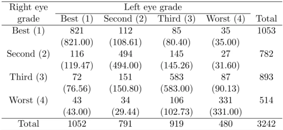
The data in Table 1, taken from Stuart (1953), are constructed from unaided distance vision of 3242 men in Britain. Table 2 gives the 7× 7 table of the diamond shape formed by rotating the data in Table 1 forty-five degrees.
The DD model fits the data poorly yielding G2 = 53.69 with 4 degrees of freedom. Also, the UADD model fits poorly yielding G2 = 51.61 with 3 degrees of freedom. However, the structure of Cov(U, V | |U|) = 0 using equally scores (i.e., w1 = w2 = 1/2) fits very well yielding G2 = 2.33 with 1
degrees of freedom. From Theorem 2.2, we see that the poor fit of the DD model is caused by the influence of lack of structure of the UADD model (not the lack of the structure of Cov(U, V | |U|) = 0).
Table 1. Unaided distance vision of 3242 men in Britain; from Stuart (1953). The parentheses values are maximum likelihood estimates of expected
frequencies under the hypothesis that Cov(U, V | |U|) = 0.
Right eye Left eye grade
grade Best (1) Second (2) Third (3) Worst (4) Total
Best (1) 821 112 85 35 1053 (821.00) (108.61) (80.40) (35.00) Second (2) 116 494 145 27 782 (119.47) (494.00) (145.26) (31.60) Third (3) 72 151 583 87 893 (76.56) (150.80) (583.00) (90.13) Worst (4) 43 34 106 331 514 (43.00) (29.44) (102.73) (331.00) Total 1052 791 919 480 3242
Table 2. The 7× 7 table of the diamond shape formed by rotating the data in Table 1 forty-five degrees.
Right eye grade minus Right eye grade plus left eye grade
left eye grade 2 3 4 5 6 7 8
−3 * * * 35 * * * −2 * * 85 * 27 * * −1 * 112 * 145 * 87 * 0 821 * 494 * 583 * 331 1 * 116 * 151 * 106 * 2 * * 72 * 34 * * 3 * * * 43 * * *
§5. Conclusion
When the DD model fits the data poorly, Theorem 2.2 may be useful for seeing the reason for the poor fit, namely, which of the lack of structure that the weighted covariance Cov(U, V | |U|) equals zero and lack of the UADD model influences strongly.
§6. Discussion
Many readers may think that the decomposition of the DD model using the structure of Cov(U, V ) equals zero, where
Cov(U, V ) = E(U V )− E(U)E(V )
= ∑ ∑ (s,t)∈S∗ stp∗st−( ∑ ∑ (s,t)∈S∗ sp∗st)( ∑ ∑ (s,t)∈S∗ tp∗st ) .
However, when the DD model holds, the structure of Cov(U, V ) = 0 does not always hold. Under the DD model, the probabilities p11, p1R, pR1and pRR are
unrestricted. On the other hand, under the structure of Cov(U, V ) = 0, these probabilities are restricted. Thus, it is difficult to consider the decomposition of the DD model using the the structure of Cov(U, V ) = 0. Therefore, in this paper, we consider the decomposition of the DD model using the weighted covariance Cov(U, V | |U|) and covariance Cov(U, V | |U| = k) in Section 2.
When we express P(U = s, V = t | {V = R + 1 − k} ∪ {V = R + 1 +
k}) as p∗∗st(k) for (s, t) ∈ S∗ and k = 1, . . . , R− 1, we can consider another weighted covariance and similar decomposition of the DD model using another conditional probabilities{p∗∗st(k)}, although the detail is omitted.
Acknowledgments
The authors would like to thank the referee for the helpful comments.
References
[1] A. Agresti, Analysis of Ordinal Categorical Data, John Wiley & Sons, New York, 1984.
[2] L. A. Goodman, Simple models for the analysis of association in cross-classifications having ordered categories, Journal of the American Statistical Association. 74 (1979), 537–552.
[3] L. A. Goodman, Association models and canonical correlation in the analysis of cross-classifications having ordered categories, Journal of the American Statisti-cal Association. 76 (1981), 320–334.
[4] L. A. Goodman, The analysis of cross-classified data having ordered and/or un-ordered categories: association models, correlation models, and asymmetry mod-els for contingency tables with or without missing entries, Annals of Statistics.
13 (1985), 10–69.
[5] A. Stuart, The estimation and comparison of strengths of association in contin-gency tables, Biometrika. 40 (1953), 105–110.
[6] S. Tomizawa, Uniform association diamond model for square contingency tables with ordered categories, Journal of the Japan Statistical Society. 24 (1994), 83– 88.
[7] S. Tomizawa, N. Miyamoto and M. Sakurai, Decomposition of independence model and separability of its test statistic for two-way contingency tables with ordered categories, Advances and Applications in Statistics. 8 (2008), 209–218.
Kiyotaka Iki
Faculty of Economics, Nihon University Chiyoda, Tokyo 101-8360, Japan