GLOBAL OPTIMIZATION PROBLEM WITH MULTIPLE REVERSE CONVEX CONSTRAINTS AND ITS APPLICATION TO OUT-OF-ROUNDNESS PROBLEM

Journal of the Operations Research Society of Japan

Vol. 39, No. 3, September 1996

GLOBAL WITH MULTIPLE

OPTIMIZATION PROBLEM

REVERSE CONVEX CONSTRAINTS AND ITS APPLICATION TO OUT-OF-ROUNDNESS PROBLEM

Yang Dai Jianming Shi Yoshitsugu Yamamoto

Kobe University of Commerce Science University of Tokyo University of Tsukuba (Received October 6, 1994; Revised April 11, 1995)

Abstract We consider a global minimization problem: min{cT-c+dT

1

-c E X , y G Y ^h, ( X , Y) â F}, where X and Y are polytopes in Rnl and Rn2, respectively; F is a closed convex set in R"~'"~; and

Gh (h = l , , . . , m 2 ) is an open convex set in Rn2. We propose an alogorithm based on a combination of polyhedral outer approximation, branch-and-bound and cutting plane techniques. We also show that the out-of-roundness problem can be solved by the algorithm.

1 Introduction

In this paper we consider the following minimization problem: min c T x + d T y

s.t. X â X ,

Y â ‚ ¬ ~ \ r j ~ (X, y) â

where X and Y are polytopes in Rnl and Rn2, respectively; F is a closed convex set in Rndn2; and Gh ( h = 1 , .

. .

,

m2) is an open convex set in Rn2; the vectors c and d are in Rnl

and Rn2, respectively. In many applications the constraints in (1.1) are usually given as a system of inequalities, then we assume in this paper that

where Ao, B. and ao, bo are matrices and vectors of appropriate sizes;

fi

(i = l,

.

.

.

,

mi) and gh ( h = 1,.

. .

,

m2) are convex functions. Obviously, the constraint y

$

uyzlGh can be rewritten as gh(y)

>.

0 for h = l,

...,

m2. The constraint gh(y)

>

0 is often called reverse convex constraint (see, e.g., Horst and Tuy [g]). By setting

Multiple Reverse Con vex Constraints

Problem (1.1) is equivalent to the following noncanonical d. c. problem:

1

min cTx

+

dTy

Note that /(-) is a convex function.

Problem (1.3) includes several important classes of global optimization problems, such as a special d.c. programming problem, a class of problems with multiplicative terms [7].

Moreover it certainly contains the canonical d.c. programming (see, e.g. Horst and Pardalos [S])

-

Recently several algorithms [4, 7, 101 are proposed for solving a special case of (1.3) in which only one additional reverse convex constraint is considered. Since a single reverse convex constraint is not available to represent the set defined by multiple reverse convex constraints, their algorithm is not directly applicable to Problem (1.3). The general branch- and-bound algorithm is a sole method for solving Problem (1.3) (section X.2 in [g]), which however does not make use of the structure of the problem. Since Problem (1.3) possesses a special structure that the reverse convex constraints are defined only on the y-space, we devise an algorithm which takes advantage of this specific structure.

Our new algorithm is based mainly on a combination of polyhedral outer approximation method and conical branch-and-bound in which the partition is made only in the y-space. Since only linear programming problems are solved in each step, it should not be costly to determine a solution for subproblem even if adding a new cut changes the feasible region. Therefore we can incorporate the cutting plane method whenever a cut is available. The algorithm can be regarded as a generalization of the first algorithm proposed in [7].

To use polyhedral outer approximation and conical subdivision we assume that ( A l ) int ((X X Y)

n

F)

#

0.

(A2)

nzl

Gh

#

0

and a point yO E

nZl

Gh is available.

Furthermore we require that the reverse convex constraints are essential, i.e.,

(A3) there exists a point (X*, y*) such that (X*, y*) E (X X Y)

n

F, y* E G and cTx*+dT

<

cTx

+

dTy for any (X, y) E W.

The remainder of this paper is organized as follows. Section 2 describes a partition of Rn^"2 based on a conical partition of Rn2. We also show how to find the lower and upper bounds in Section 2. Section 3 gives the algorithm and proves its convergence. In Section 4 we show that the out-of-roundness problem [ l , 111 can be formulated as Problem (1.3) and describe the details of the method for obtaining the lower and upper bounds for this specific problem.

2 Branching and bounding operations

We establish a subdivision underlying the branch-and-bound algorithm in this paper. Owing to the special structure of the problem we first subdivide the subspace Rn2 and then build the subdivision on the whole space We use a conical partition as the subdivision of the subspace Rn2. The bounding operations are carried out by solving a series of linear programming problems.

2.1 Conical partition

Let yO,

z'

(i = l,

...,

n2) be n2

+

1 affinely independent points of Rn2. We call the convex polyhedral cone { y E Rn2

\

y =

2

(2' - yO)

+

yO,

2

>

0 } the cone generated by points yO, zl,

...,

zn2. The cone has exactly n2 edges emanating from point yO. Without

358 Y. Dai, J. Shi & Y. Yamamoto

loss of generality, we assume that all zz are on the surface of the unit ball B(yO) = { z E Rn2

I

11

2 - y0

11

1

l } with center at go.

For a subset Y' & Rn2 a collection C of finitely many cones { Cl,

...,

Ct } defined above is called a conical partition (see figure 1) of Y' if u & ~ C ~ = Y' and int Ci

n

int Cj =

0

for i

#

j .

We also call a collection V = { D l ,

. . .

,

Dt }, where D j = Rnl X C,, a conical partition of

Rnl X Y'.

Let C and C' be conical partitions of Rn2. Conical partition C' is said to be a refinement of C if for any C' G C' there exists a cone C G C such that C" C.

In our algorithm we repeatedly refine the conical partition of Rn2 to yield a sequence {Ck }k=1,2, of conical partitions. The refinement process is called exhaustive if for every strictly nested sequence { C"k }k=1,2,... satisfying Ck G Ck and Ck+i C Ck for every k , there exists a vector 2 on B(yO) such that

lim z\ =

z

for all i = 1,

...,

n2. k+oo

Figure 1: Conical Partition

2.2 Lower and upper bounds

Let P be a polytope containing all optimal solutions of (1.3), e.g., one can take X X Y

as P. Then we can assume without loss of generality that P is contained in X X Y. Let

V = { Dl,

. . .

,

Dt } be a conical partition of R"'+"'. We consider how t o compute a lower bound Lj of cTx

+

dTy over ( P

n

W)

n

D j = ( P n W )

n

(Rnl X C'.) for j = 1,.

.

.

,t.

For the sake of brevity, we omit the subscript j and let D = Rnl X C denote a cone of the conical

partition V = {

D i ,

. . .

,

Dt

}

throughout this and next subsections.

Assume that the polytope P is defined by the following system of inequalities:

where A, B, and b are matrices and a vector of appropriate sizes. Note that P does not necessarily contain the whole set (X X Y) F. We propose a procedure for calculating the

lower bound L of cTx

+

dTy over the set P

n

W

n

D.

For the cone C determined by go, zl,

...,

zn2

,

let 6 = 2 max{9

1

y0

+

9(z - yO) G Y, z

c

B(gO) } and let

(2.1)

e h

= min{ 9, sup{@

I

y0

+

9(z' - yO) G Gh }} for i = 1,

...,

n ~ . And define for every Gh (h = 1,.

. .

,

m ^ ) a set of n2 points

Multiple Reverse Convex Constraints 359

We denote by Oh the ^-dimensional vector ( O l h ,

...,

en2h)T,

Uh the n2 X n2-matrix (vlh - yO,

. .

,

vnzh - {Y'). Define a half space Hh in Rn2 as

Hh = { { Y E Rn2

l y =

yO+uhAh,eT\'Â¥ l},

where e = (1,

...,

l) T. From the choices of y0 and v l h ,

..

.,

Uh is a nonsingular matrix, then Hh can be written as

Then the intersection of and the cone C is written as

and for every point (X, y) E P

n

(Rn1 X

nzl

Hh) f l D , there exist nonnegative vectors

Ah = (A1*,

...,v

for h = 1,

...,

mi, such that eTAh

>

1 and

Lemma 2.1 For every (X, y) E P

n

(Rn1 X

n z l H h ) n

D, Ah in (2.4) is bounded for

h = 1,

...,

7722.

Proof. Let h be an arbitrary index of {l,

...,

m2}. From (2.4) point y with (X, y) E P

n

(Rn1 X n',"zlHh)

n

D is written as

that is

Ah =

(u~)-'({Y

- yO).

Then we obtain

l

Ah

l l

^

ll

(^'Â¥)-

l l l l

Y - {YO

11,

which is bounded since y is in the polytope Y.

Let

The following lemma shows that L is a lower bound of cTx

+

dTy over the set P

n

W

n

D .

Lemma 2.2

(i) If P

n

(Rn1 X

n z l H h )

n

D is empty, then the optimal solution of (1.3) is not zn

P n W n D .

(it) If P

n

(Rn1 X

n ; " ~ ~ )

n

D is not empty, then

~ < , m i n { c ~ x + d ~ y \ ( x , ~ ) E P n W n D } .

Proof. From the definitions of H h , C and G, we see that { y

1

y @ G }

n

C

C

(nrzlHh)

n

C , then

360 Y. Dai, .l. Shi & Y. Yamamoto

Therefore we obtain (ii). Moreover if P

n

(Rn1 X n;";,Hh)

n

D =

0,

then P

n

W

n

D =

0.

It implies (2).

From the above lemma, it seems that we have to solve a linear program with a lot of linear constraints when m2 is large. However from Lemma 2.3 below, it is likely that we can remove many of such constraints of Hh ft C in computing (2.5).

Lemma 2.3 For h,, h, E {l,.

. .

, m 2 } if Shl

>

Sh2) then H^ ft C

C

H^

n

C.

Proof. Let y be a point of Hhl

n

C, then there exists a vector

X^

>

0 such t h a t eTX^

>

1 and

Let tz = Szh1/@h2, which is well defined by Sih2

>

0, then ti

>

1 and we obtain

Note that tiAzhl

>

0 for all i and

E

tiAihl

>

l. This means y ? Hh2 Cl C.

The following lemma is derived from Assumption (A3).

Lemma 2.4 Let (X*, y*) be a global optimal solution of (1.3)) then y* is on the bound- ary of G.

Proof. Suppose that the optimal solution (X*, y*) of (1.3) is not on the boundary of G.

Then gh(y*)

>

0 for any h E {l, . .

.

,

m,}. Let (X(\), y(A)) = (A(x*, y*)

+

(1 - \)(X*, y*)) for (X*, g*) of Assumption (A3). Then for any A E (0, l]

cTx(A)

+

dT y(A)

<

cTx*

+

dT y*.

Therefore cTx(A)

+

dT y(\)'< cTx*

+

dT y* for some

A

E (0, l] and gh (y(A))

>

0 for all h. By the convexity of X, Y and F, we also see that X('\) E X, y(\) E Y and (x(A), y(A))

c

F. I t implies that (X(\}, y(X}} is a feasible solution of (1.3). This is a contradiction.

After solving the linear programming problem of (2.5) we obtain an optimal solution (3, g) and the corresponding objective function value L. If the point (3,

g)

lies in P fl W , it is a n optimal solution of min{ cTx

+

dTy \{X, y) E P

n

W

n

D }. Then the currently considered

D need not be subdivided further. Moreover, L serves as an upper bound of the optimal value of Problem (1.3).

If (3,

y}

4

P

n

W , then we possibly find a feasible point of (1.3) by moving from (3, jj) along some specific direction. A possible choice of the direction is (c, d). Let

and define a point (X,

y)

by

(2.7) (X, y) = (X, jj)

+

+(C, d ) .

If (X, y) E W , then the value cTX

+

dT is an upper bound of the optimal value of (1.3). If (X, y)

9

W , then it is difficult in general t o find a feasible point of (1.3) by moving ( 2 , y). T h e

Multiple Reverse Convex Constraints

following technique, however, works well, for example, for the case of the out-of-roundness problem in Section 4. Namely we fix y and search a test point. Let

and let

A

= sup{-\

1

[(it, y), (it

+

\ ( X - it),

y)]

n

(X X Y)

n

F = 0}, where [ S ,

-1

stands for a

closed line segment. If

A

<

+m, then we let the test point (2,

6)

be determined by

Lemma 2.5 If

A

<

+m, then

(5,g

6 (X X Y)

n

F .

Proof. Suppose (2, y)

4.

( X X Y) F. Then we have

By virtue of compactness of (X X Y) f1 F, there exists E

>

0 such that

It contradicts the definition of

A.

2.3 Polyhedral outer approximation and cutting plane

At the beginning of the algorithm, we take the polytope X X Y as a n initial polytope Pi

containing ( X X Y)

n

F. The algorithm generates a sequence of polytopes { Pk

1

fc = 1,2, ...}

such that Pi 2 Pa and each Pk contains an optimal solution of (1.3).

At the kth iteration, we construct a conical partition over some cone D chosen in the (k- 1)st iteration. By solving linear programming problem (2.5) for all cones in the partition, we obtain several lower bounds. We also obtain several, possibly no, feasible points of (1.3), which are generated by solving (2.5) or by (2.7)-(2.9). After bounding operations (see Section 3 for the details) we choose a point with minimal lower bound t o obtain a point ( z k , yk), which is an optimal solution of (2.5) for some cone of D. If we find some feasible points, then choose one of them, say (X,

y}

having the smallest objective function value. We can take the inequality

(2.10) cTx

+

dTy

<

cTx

+

dTiJ

as a cutting plane if the value cTx

+

dT

iJ

is less than the current upper bound. Adding (2.10) t o the constraints of PI: will not cut off the optimal solution of (1.3). Moreover, if

(zk,

gk) f F , compute a subgradient S ( z k ,

yk)

of f a t ( z k , tt,) and let

Then the inequality

(2.12) l k ( ~ , Y)

5

0

will cut off the point

(zk,

yk) but no feasible points of (1.3) in Pk. Therefore we can define the polytope Pk+i for the next iteration by

However, on the situation that only one of the cutting planes (2.10) and (2.12) or no cutting planes can be constructed, Pk+i is defined by adding the corresponding cutting plane t o Pk or by Pk+i = P k , respectively. The latter occurs if ( z k , yk) E F

n

G.

362 Y. Dai, J. Shi & Y. Yamamoto

3 Algorithm

Based on the above discussion we propose an algorithm for solving Problem (1.3) as follows. Algorithm

begin

Construct a polytope Pi : Pi

2

W and a conical partition C of Rn2;

M\ := C ; 7 := +m; k := 1;

while M k

#

0

do begin

for each C E M k do begin

Solve linear program (2.5) ;

( x ( C ) ) g(C)) := the optimal solution; L(C) := cT3(C)

+

dTg(C); if ( z ( C ) ) @ ( C ) ) E W and 7

>

 £ ( C then begin 7 := L(C);

(0)

:=

( ~ ( c ) )

y(C)) end else begin Compute ( 2 , y) by (2.7);

if ( i 7 y ) E W and 7

>

cTit+dTy then begin 7 := cTit+dTy; ( X , y ) := (it, y ) end else begin Compute ( 5 ) y ) by (2.8) with (2.9); if (5, y ) E W and 7

>

cT5

+

d T y then begin 7 := cT5

+

d T Y ; ( X )

y )

:= ( 5 ) y) end. end end end; if { C e M k 1 L ( C ) < 7 } # 0 t h e n M k + l : = { C â ‚ ¬ M k l L ( ( ? ) < else goto Out-of- while ;

Choose a set C E Mk+i satisfying cTx(C)

+

dTy(C) = min{ L(C)

1

C E Mini }; Ck := C ; ( x k ) y k ) := @(Ck), ~ ( c k ) ) ;

if 7 is updated then Pk+1 := Pk n { ( X ) y )

\

cTx

+

d T y

5

7 }

else Pk+1 := Pk;

if

( z k ,

ok)

<i

F then

begin

l k := [ ( X ) Y ) - ( x k , ~ k

]s(xk

) 7 y k )

+

f

( x k ) %) 5 0;

Pk+1 := Pk+l

n

{ ( X , Y )

I

zk(x, Y ) 5 0 }

end

Construct a conical partition Ck of Ck; Mk+1 := Mk+l

\

{ Ck } U C k ; k := k

+

l

Multiple Reverse Con vex Constraints

Out- of- while ;

if 7 := +m then writeln(' The problem is infeasible ')

else writeln(' The solution is

',

( X , y))

e n d .

3.1 P r o o f of the validity of t h e a l g o r i t h m

If the algorithm terminates within a finite number of iterations and 7

<

+m, then clearly we obtain an optimal solution of Problem (1.3). If it terminates with 7 = +m, we see that the problem has no feasible solution.

T h e o r e m 3.1 If y = +m when the algorithm terminates, the problem (1.3) has n o feasible solution.

Proof. Note that the algorithm terminates only if

Mk+l

becomes vacant and that it has two steps where

Mk

is updated:

and (3.2)

Since

Mk+l

does not become vacant at Step (3.2), we conclude that

meaning (2.5) is infeasible for any C E M t . Suppose (1.3) has a feasible solution, say (X, y). Then it is feasible for (2.5), and hence L(C) is finite if and only if the corresponding cone C contains y. Since 7 = +m throughout the execution of the algorithm,

Mk

keeps a cone, say C' containing (X, y). This implies that L(C1) is finite, which contradicts (3.3).

Suppose that an infinite sequence { (G, jjk) }k=1,2,... is generated by the algorithm. Since the sequence is in compact set X X Y, and hence bounded, it has a cluster point (X*, g*) E X X Y. We see that the conical partition Ck consists of finitely many cones, therefore there exists a t least one cone of Ck containing infinitely many points of (G yk). Consequently, we can choose a subsequence { ( 3 k q ,

gkq)

}q^i,2,... of the above sequence and a sequence {Ckq}q=1,2,.. of nested cones such that

( z k ,

j j k ) E Ckq

.

The following two cases can happen.

Case(1) there exists a such that for all q

>

q, (£kq

ykq)

6 F ; Case(2) for any q there exists q

>

q such that ( z k , j j k )

6

F .

In order to prove the convergence of the algorithm we first prove (X*, y*) C F. If case (1)

happens, then clearly (X*, y*) E F. Therefore we only consider case (2). For simplicity we assume that the points

( x k ,

y k )

does not belong to F for every q by taking a suitable subse- quence of {

(xi,,

)&f

}

if necessary. For a positive E let us introduce a closed E-neighborhood P(&) of Pi, i.e.,

Then

Pi

W(&).

L e m m a 3.2 T h e cutting plane functions { Lkq }o=l,2,... are uniformly equicontinuous o n p1

364 Y. Dai, .l. Shi & Y. Yamamoto

Proof. From the compactness of P ( & ) we see that the convex function f ( X , y) is bounded

on P ( & ) , i.e., f ( X , y)

<

M for some M . By the definition of subgradient

and consequently

holds for all ( X , y) E P ( & ) and for all k . Suppose that { S ( z k q , f i q )

1

q = 1,2,

...

} is

unbounded, then there exists a t least one unbounded component of S ( x k q ,

y k ) .

We as- sume without loss of generality that the first component of S ( Z k q ,

vie)

is unbounded. By

(zkq,

j j k q ) E Pi, we can take a point ( X , y) E P ( & ) such that ( X , y) - (ikq, ykq) = ( h e , 0,

...,

0 ) .

By choosing an appropriate sign of E , we have [ ( X , y) - ( x i , , t/kq)]S(?kq,

yic}

>

M for a suf- ficiently large q, a contradiction to (3.4). Therefore { S ( x k q 7 % )

1

q = 1,2,

. . .

} is bounded.

Let M17 M2 and Ms be sufficiently large numbers such t h a t

11

( X , y) - ( G

aq)

11

<

M i ,

11

S ( Z k q ,

ykq)

1 1

5

M2 and

1

f ( X , y)l

5

M3 hold for all ( X , y) E Pi and for all q. Then

llkq(x, y)l is bounded by M1M2

+

M3 for all ( X , y) E Pi and for all q. Therefore, both

sup{ lkq ( X , y) \ { X , y) E Pi, q = 1,2,

...

} and inf{ L { x , y) \ { X , y) E Pi, q = 1,2,

...

} are finite.

The desired result follows from Theorem 10.6 of [13]. 0

Since { lkq ( X , y)

\

( X , y) E Pi, q = 1,2,

...

} is bounded, by Theorem 10.8 of [ I s ] , lk,

,

lk,,

...

converge uniformly to a continuous function l , i.e.,

lim sup \lkq ( X , y) - l ( x , y)

\

= 0.

(X,Y)€

We have

Lemma 3.3 lim l t q ( z i q 7 i ~= l(x\ ~ )Y * ) .

9-

Proof. Since l k converges uniformly t o l , we have that for every e

>

0 there exists qi such

that

From lim

( x i , ,

gkq)

= ( X * , y*) and the continuity of l , we have lim l(Zkq

,

j j k ) = l ( x * , y*), i.e.,

9+rn 9 - + ~

for every E

>

0 there exists q2 such that

Then we have for all q

>

max{ ql, q2 },

Multiple Reverse Convex Constraints

By the boundedness of S ( x k q , y k q ) , we can find a subsequence of S ( x k q ,

gkq)

converging t o a vector S. Therefore

l ( x , Y ) = [ ( x , y ) - ( X * , Y * ) I S

+

f{x*> Y * ) ,

implying f ( X * , y*) = l ( X * , y*). By the definition of F, we have the lemma.

Lemma 3.5 _{lkq ( x k q + ~ 9 k q + ~ ) = l ( x * Y * )} q-+*

Proof. By lim lkq (Zkq, ykq) _oÑfo = l ( X * , y * ) and lim ( g k q , j j k ) = ( X * , y * ) , we see that for every

q-+w E

>

0 there exists q1 such that

and for every 8

>

0 there exists q2 such that

From Lemma 3.2, we see t h a t { l k q ( x , y ) } is equicontinuous a t ( X * , y * ) , i.e., for every E

>

0 there exists 8

>

0 such that

Therefore for every e

>

0 we have that for q

>

m a x { q i , q2 }

Theorem 3.6 ( X * , y * ) E F .

Proof. Note that kq+l

2

k q + l . Then by the definition of (a;kq+l,

& + ) ,

we see

( z k ,

ykq+i)

^tq+l

c

Pkq+i, meaning

4,

(Â¥ftq+l 2/iq+l)

5

0. Therefore l ( X * , y*) <_ 0 by Lemma 3.5. Then

Lemma 3.4 proves the assertion. D

We have proved that every cluster point of the sequence { Z k ,

yk}

generated by the algorithm belongs to F. Moreover, from Pk

C

X X Y for k = 1 , 2

...

we have ( X * , y*) E

( X X Y ) H F .

Theorem 3.7 Suppose the conical partitions generated by the algorithm are exhaustive.

If

7

< +m

t h e n every cluster point of the sequence { (& y k ) } i s a n optimal solution of Problem (1.3).

Proof. Let ( X * , y*) be a cluster point of

{

(G

ijk)

}.

Assume t h a t

{

( x k ,

i j k )

}

is a sub-

sequence of {

( x k ,

&) } converging to ( X * , y*) such that ( g k q , ykq) E Dkq = Rnl X C k for a

366 Y. Dai, l. Shi & Y. Yamamoto

First we show y* if. G . From the assumption that { C k q } is exhaustive, there exists a vector Z 6 Rn2 such that y* is on the ray { y

\

y = y0

+

9 ( ~ - y O ) , 9

2

O}. On the other

hand, by the definitions of

( z k ,

i j k ) and C k

,

where e T \ ^

>,

1 and

\^

>

0. From the definition of u p in (2.2) ( where index kg is omitted

) we see that

By Lemma 2.1, we have that { A ;

\

h = l ,

...,

m2, q = 1,2,

...

} is also bounded. Taking a subsequence if necessary, we obtain that

lim @h = P h , lim ~ i h = >Â¥

q+m kq q+m ^1 for i = 1,

...,

n2 and

Aih

2

1 ,

A"'

>

0.

Hence

nz

(3.6) = y O + ( z - y 0 ) E 9 A -ih i h for all h .

1=1

Suppose y* E G, then there exists a t least one h. such that y* G Gho. We will show t h a t (3.7) y0

+

P h o ( 2 - yO) G 3Gho for some i.

Suppose that y0

+

phO

( 2 - yO) if. 3Gh0 for all 2 . Note that 9 9 is taken either as 0 in (2.1)

or such that yO

+

Q ( z ; - y O ) E 9Gh0. Then for sufficiently large q

which implies

P

= C for all i.

Therefore from (3.6) we obtain

From the definition of

e,

(3.8) contradicts the fact that y* G Y. Therefore (3.7) holds true. Moreover, it follows that from the compactness of 3Gho

(3.9) y0

+

e""'(Z - yO) G 3Gh0 while

PhO

#

C for all i.

Taking fth0 = rnin

PhO,

by virtue of (3.7) and (3.9), we see t h a t y0

+

fth0 ( Z - yO) E 9Gho.

From y* E Gho therefore

x9'h0xh

<

fthO = mjnmhO. On the other hand, ~ f f ' h O ~ i h O

?.

E

fthOiihO

>

f f h O , a contradiction. It implies that y*

if.

G.

Combining the above result with Theorem 3.6 we see t h a t (X*, y*) is a feasible solution of Problem (1.3), i.e., ( X * , y*) E W .

Let V* be the optimal value of (1.3). Note that c T z k

+

dTfjkq is a lower bound of V*, therefore we see that

Multiple Re verse Con vex Constraints 367

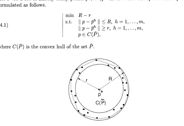
4 Out-of-roundness problem

Let P be a set of finitely many points pl,

. . .

,

p"1 in R". T h e out-of-roundness problem is formulated as follows.

min R - r

s.t.

_{[ I p - p h 11}

_{$ R , h = 1 , . . . , m ,} p - p h

11

> . r , h = l ,

...,

m, P E C ( P ) ,

where C ( P ) is the convex hull of the set P.

Figure 2: Out-of-Roundness Problem

The problem is to find a pair of concentric balls one of which contains all the points

$,

.

.

. ,p- and the other contains none of them such that the difference of two radii is minimized. If the objective function R - r is small enough, we can conclude t h a t the given points p',

. . .

lie on the surface of a ball.

There are several algorithms [l, 111 dealing with the problem. The proposed algorithms

[l, 111 can solve 2-dimensional out-of-roundness problems in 0 ( m 2 ) time. To the authors' knowledge there are no algorithms developed for solving problems with dimensions higher than two. The algorithms in [l, 111 are based on constructing the nearest and furthest neighbor Voronoi diagrams. However, constructing the nearest neighbor Voronoi diagrams alone needs 0 ( m w 1 ) time, which increases exponentially with the dimension n (see 121). Moreover, whether the approaches in [l, 111 can be generalized to solve problems with n

>

2 is not clear. In the remaining part of this section we show that the out-of-roundness problem can be formulated as Problem (1.3), where the structures of X, Y, F and G of constraint sets are rather simple. By taking advantages of the structures, we show t h a t the algorithm proposed in the previous section can be applied efficiently t o the problem.

We consider the problem (4.1) with the last constraint p E C ( P ) dropped, i.e., min R - r

. t .

_lip-ph

₁₁

_{5 R , h = !}

_{, . . . ,}

_m,

11

> r , h = 1 , . . . , m .

In practice the given points

p ,

.

. .

, p

represent the location of sample points on the surface of an almost round object. Therefore it is very likely that the solution of (4.2) lies somewhere in the convex hull of P. Let us set an assumption as follows:

368 Y. Dai, I. Shi & Y. Yamamoto

Assumption 4.1 The optimal solution of (4.2) is i n the convex hull C ( P ) .

The out-of-roundness problem is equivalent to Problem (4.2) under Assumption (4.1). Let

where ei is a j t h unit vector in R". Further we define

and consider

min R - r

s.t. R e X , ( r , p ) E Y ,

( R , r , p ) 6 F, ( 7 - , P ) P+' \G.

is an open convex set. The polytope X is just an interval and the polytope Y is a hypercube of dimension n

+

1. From the nature of this problem the ratio of m / n is usually very large.

Theorem 4.2 Under Assumption 4.1 the problems (4.2) and (4.3) are equivalent.

Proof. Let (R* (2 ) , r* ( 2 ) , p* ( 2 ) ) and (R* ( 3 ) , r* ( 3 ) , p* ( 3 ) ) be optimal solutions of Problem (4.2) and Problem (4.3), respectively. Since (R* ( 3 ) , r* ( 3 ) , p* ( 3 ) ) is a feasible point of the

problem (4.2),

(4.4) R'(2) - r * ( 2 )

5

R * ( 3 ) - ~ ' ( 3 ) .

On the other hand, we obtain p*(2) =

E ; "

A l p h for some nonnegative A; such that

S=,

A; = 1 from Assumption 4.1 and R* ( 2 ) =

11

p* ( 2 ) -

phl

11

for some

hi

E { l ,

. . .

,

m}. Therefore

Multiple Reverse Con vex Constraints 369

Furthermore, p* (2) E C(P) implies a,Â

5

p,'(2)

5

8

for j = l,

.

. .

,

n. Therefore (R* (2)) r* (2)) p* (2)) is a feasible point of Problem (4.3). Then we have

(4.5) R*(3) - r'(3)

5

R*(2) - r*(2).

From Assumption 4.1 and Theorem 4.2, the out-of-roundness problem is equivalent t o Problem (4.3)) which is solvable by the algorithm proposed in Section 3.

To start the algorithm we choose X X Y as an initial polytope Pi containing (X X Y)

nF,

where (X X Y)

n

F is defined as before. Take rO to be any value greater than pO =

max

l]

p0 - jih

11.

Then the point ( r O , p O ) belongs to n;",,Gh, and can serve as point y0 of

h

the algorithm.

Suppose that we are a t the Ath iteration of the algorithm, let the polytope Pk be defined by

Pk = { ( R , r , p ) l a t ~ + a ; r

+

~ i

<

pbk},

where a*, a: and bk are m"-dimensional vectors, and B* is an mk X n-matrix. To obtain

a lower bound over a set Pk

n

W

n

D, let ( r l , p'),

.

.

.

,

(rn+l, p"+') be points generating the cone C . Since each constraint gh(r,p)

<

0 defining the set G h is very simple, a solution of the equation

11

p0

+

Oih(p2 - pO) - ph

11

- (rO

+

$"'(ri - To)) = 0,

if any yields the value of

9th,

for which (r2h, pih) = ( r O , pO)

+

$^(r2 - r O , pi - p') lies on the

intersection of 9Gh and the zth ray of the cone C. After computing the set of n

+

1 points (rih)pih)).

.

.

,

(rn+lyh,pn+lyh) for every h (h = 1 , .

.

. , m ) , we have to solve a linear program (2.5) to obtain a lower bound and possibly an upper bound. The linear program (2.5) can be written as (4.6) min s.t. Recall Uh = [(rlh - rO,pl" - p'), then r

=r0++Y,

Vh, p = p 0 + + * Vh.

Take an arbitrary number of { 1 , .

.

.

,

m}, for instance 1 and substitute (4.7) and (4.8) with h = 1 for r and p of (4.6)) respectively. Then the problem (4.6) reduces t o

(4.9) min R -

U i P

- r O ~ . t .

a k ~ +

B k \ l ^

P,

(/"A* - U ' A ~ = 0, A = 2 , . .

.

, m , eTAh

>

1, h = 1,

...,

m, * R

>

0, h = 1 , . . . , m ,

370

where

Y. Dai, J. Shi & Y. Yamamoto

The above problem has mk

+

( n

+

l ) ( m - 1)

+

m constraints and ( n

+

1)m

+

1 variables, and the number mk grows a t each iteration as cutting planes are introduced. Therefore it is time consuming to solve this problem directly. We deal with this shortcoming as follows. There are lots of redundant constraints in (4.9). Using Lemma 2.3 we can remove h from the set { 1,

..,

m } if there exists an h' such that Oh'

<

Oh. Let I be the remaining subset of

{ 1,

..,

m } after removing all those h, relabel the elements in I as 1,

.

.

.

,111, and relabel also correspondingly Uh and Xh. We consider the dual problem of (4.9). Let

C,

$,

. . .

,

t?lI1-l, [ be dual variables of the reduced and relabeled problem (4.9), where

C

is a vector of mk- dimension, f l ,

.

. .

,

n ^ l l are vectors of (n

+

l)-dimension, and $ is a vector of (11-dimension.

The dual problem is max

1

s.t.

Note that the above problem has (n

+

1)lIl+ 1 constraints. It is obvious that solving (4.10) is less time consuming in comparison with solving (4.9) directly.

The other thing worth mentioning is that the methods of finding possible feasible points in (2.7) and (2.8)-(2.9) are extremely simple. By solving (4.10) we obtain a point (R, f ,

p).

Suppose (R, f,p)

6

( X X Y ) F. Then

1

p - p h

11

- F < 0 for h = l , . . . , m .

The value of f = sup{ T

1

r d

+

y

E G } in (2.7), where d = (- 1, O), y = (f, p), can be

determined by

f = max{f -

11

p

-

ph

11

\

h = 1,.

. .

, m } .

In fact the point ( f d

+

g) = (f - F, p) belongs to G , since

and a t least one equation holds. Then the point (?,c) = (R, F,

p)

in (2.7) can be determined by ?(c, d)

+

( 3 ,

y}

= ?(l, - 1 , O )

+

(R, F ,

p).

If the point

(?,c)

= (h,?,?) in (2.8) is necessary, we have to determine first X = R satisfying (2.9), i.e., to solve the following maximization problem

Note that ( R , r , p ) E Pk satisfies 0

5

R

<

2p0. Therefore (4.11) has an optimal solution. The optimal solution is simply given by

Multiplc Rcver,sc Con vex ConLstraints 3 71

5 Conclusions

We have proposed an algorithm for solving the global optimization problem with a set of reverse convex constraints by means of cutting plane techniques and branch-and-bound method. The out-of-roundness problem has been discussed as a special case of the problem considered in this paper. The techniques proposed to find a feasible point in (2.7)-(2.9) become very simple when applied to the out-of-roundness problem. The proposed method formulating a computational geometry problem as a global optimization problem is also suc- cessful for the largest e m p t y sphere problem (see Shi and Yamamoto [3]). This is a concrete example using continuous approaches to discrete optimization problems (see Pardalos [12]). References

H. Ebara, N. F'ukuyama7 H. Nakano and Y. Nakanishi? A practical algorithm for computing the roundness, IEICE Trans. Inf & Syst. E75-D (1992) 253-257.

H. Edelsbrunner? Algorithms in Combinatorial Geometry7 Springer-Verlag, 1987.

J . Shi and Y. Yamamoto, A d.c. approach to the largest empty sphere problem in higher dimension, in: C.A. F'loudas and P.M. Pardalos eds., State of The Art in Global Optimization: Computational Methods and Applications, Kluwer Academic Publishers (1996) 395-411.

R. Horst, T.Q. Phong and N.V. Thoai, On solving general reverse convex programming problems by a sequence of linear programs and line searches7 Annals o f Operations Research 25 (1990) 1-18.

R. Horst and P.M. Pardalos? Handbook o f Global Optimization, Kluwer Academic Publishers, 1995.

R. Horst and N .V. Thoai, Modification, implement ation and comparison of three algorithms for solving linearly constrained concave minimization problems, Computing

42 (1989) 271-289.

R. Horst and N.V. Thoai, Constraint decomposition algorithms in global optimization,

Journal o f Global Optimization 5 (1994) 333-348.

R. Horst, N.V. Thoai and H.P. Benson, Concave minimization via conical partitions and polyhedral outer approximation, Mathematical Programming 50 (199 l ) 259-274.

R. Horst and H. Tuy, Global Optimization : Deterministic Approaches, Springer-Verlag, 1993.

T . Kuno and Y. Yamamoto, A parametric simplex algorithm for solving a class of rank-two reverse convex programs, Research Report, ISE-TR-93-1037 University of Tsukuba, 1993.

V.B. Le and D.T. Lee, Out-of-roundness problem revisited, IEEE Trans. Pattern Analysis and Intelligence 13 (1991) 217-223.

P.M. Pardalos, Continuous approaches to discrete optimuzation problems, in: G. D. Pi110 and F. Giannessi eds. Nonlinear Optimization and Applications, Plenum Publishing (1996) 313-328.

R.T. Rockafellar, Convex Analysis Princeton University Press, 1972.

Yoshitsugu YAMAMOTO Institute of Policy and Planning Sciences University of Tsukuba Tsukuba, Ibaraki 305, Japan E-mail: [email protected]