The performance of the Thai economy after the financial crisis in 1997 has induced economists, and policymakers believe that Thailand was trapped in the middle-income range. This paper reviews the stylized facts. Here, we have constructed an economic chronology of Thailand to explain the past unstable growth path. It is an impact of the external shock of currency realignment in 1985, as well as financial crises in 1997 which may have implications of the capital deepening in Thailand.
We have surveyed the theoretical as well as sought empirical evidence to explain why Thailand has been falling into the trap. Firstly, we have applied an Input-Output Table of Thailand 1975-2010 which condensed the inter-industrial relationship into 5 disaggregate sectors. With calibrated capital stock, labor employment, we have statistically analyzed the path of economic growth, capital accumulation, and factors distribution of income in Thailand in the past decades 1970s-2000s. We have tried also to explain the growth and income distribution in Thailand from various theoretical perspectives, especially the debates on capital and distribution between the Neo-Classical and Post-Keynesian schools of thought.
In the long-run, if Thailand would aim to exit from the ‘middle-income trap’, she may have to emphasize the proper level of capital accumulation. With the Ramsey-Cass-Koopmans (RCK) model simulation, we try to forecast the long-term path of capital accumulation in Thailand. It is found that the steady-state growth path of capital accumulation and consumption would be still far from reached by our current effort in capital investment. The sacrifice of current consumption would be needed to increase the saving rate for capital accumulation and steady-state growth.
The Keynesian model of growth has proved to be well behaved in the case of Thailand. The profit rate was determined by the saving rate and the capital-output ratio. The profit-wage rate ratio determines the income distribution along with capital accumulation. It has been observed that Thailand had low productivity of capital and declining profit rate overtime. On the contrary, Thailand had real wage rate growth and an acceptable labor productivity record. Thus, the income distribution worked in favor of wage earners over time rather than the profit earner like capitalists or entrepreneurs. This is contradicting to the conventional belief that exploited labor surplus was a source of capital accumulation and growth.
We, therefore, postulate that the Kuznets’ Inverted U-Shape hypothesis may be realized in the case of the Thai economy i.e., Thailand has entered the phase of a reduction of poverty as well as income inequality in recent years. However, the result of the endogenously determined saving rate by the RCK model simulation has confirmed that the Thai economy is still far from reaching the steady-state level of economic growth and equitable income distribution as had been achieved by other predecessors.
Keywords: Growth and income distribution, capital controversy, RCK steady-state growth path JEL O41
1
Kitti Limskul is a professor of Economics, Faculty of Economics, Saitama University, [email protected]
Kitti Limskul 1 Abstract
《論 文》
Economic Growth and Income Distribution:
A Debate on Capital Accumulation in Thailand
1. Introduction
The macro-economic performance in Thailand has been subjected to a business cycle for several epochs. The growth record was quite impressive except during the Asian Financial Crisis in 1997-1998.
The sources of growth from the supply side according to the growth accounting have shown that Thailand has reached the status of a middle-income country. The structural change in terms of value-added share has shifted from agriculture to the manufacturing and service sectors. The sources of growth were mainly from the capitalization deepening, rather owing to the growth of Total Factor Productivity (TFP).
Since 1972, the contribution from labor numbers and land to economic growth has declined.
The objective of this paper is to apply the economic growth model to explain the Thai economy since the 1970s-2010s. We want to find out empirically why Thailand could not get out of the middle-income trap? Thailand has taken-off from subsistence since the early 1960s and has passed economic and financial crisis in 1997. It is hypothesized that Thailand should be able to reach a stable middle-high income country in the 2000s and onward. But this has never been achieved. What has been the obstruction to the capital accumulation and growth episode in Thailand?
To analyze the cause and trying to answer the above puzzle, we have first constructed a growth accounting on the supply side. We have compiled sources of growth from capital and labor inputs weighted by their value shares respectively. Besides, to factor inputs’ contribution to the growth of output (represented by the Gross Domestic Product in constant prices), we have measured the source of growth from the technology named the ’Total Factor Productivity’.
Further, we would like to test the hypothesis that Thailand has had over capital accumulation before the Asian Financial Crisis (AFC) in 1997. It was pointed out by eminent economists especially Paul Krugman 2 that over capital deepening in East Asian economies including Thailand was inefficient. The sources of growth were biased by the inefficient capital input and caused low growth in TFP. To prove this, we have compiled a series of Input-Output accounting from the I-O Table of Thailand 1975-2020.
This is to prove whether production function, capital intensity, and factor-price frontier (in constant price) are well-behaved as assumed by the Neoclassical Theory or not? In short, it is to prove that the growth of productivity of capital before AFC was low or inefficient and maybe a fundamental source of the economic and financial crisis that occurred in Thailand. The contagion effect was later spilled over to other East Asian Economies.
In the second attempt, we would like to debate concerning the path of economic growth and capitalization trend of Thailand after the AFC 1997. We hypothesize that Thailand was undercapitalization, as the capital stock was damaged by the crash in 1997. It was not restored to its sustainable level and induced the economic growth path lower than the growth potential. This may be one of the reasons why Thailand could not exit from the middle-income trap dilemma. Here, we have applied the ‘Ramsey-Cass- Koopmans, RCK’ model to analyze the long-term optimal growth path. Given heuristic assumption on model parameters and calibration, we simulate how Thailand can reach the long-run steady-state with an endogenous response of saving and capital accumulation.
It should be noted that the study on capital accumulation in Thailand was written by eminent economists before. The pioneering work was well written by Suehiro (1989) 3 . The study was fundamentally a historical record of the emergence of the capitalist class in Thailand from 1855-1985.
The book was well informed with very impressive historical records. It was cited by most Thai study scholars. We have taken for granted that the book was a pioneering study from a historic point of analysis. In our study, we would rather choose to follow the economic approach from the philosophy of Classical, Neo-Classical, and Keynesian schools respectively. This study has chosen epoch of development of Thailand dating from 1975-2010 since we rely on the inter-industrial Input-Output accounts of Thailand. Our study, although it has a different academic path it may add on macroeconomic perspective to the previous study. We have further analyzed the income distribution in Thailand. We have applied the concept of factor incomes to lay the ground for further debates on the results.
2
Krugman, P. (1994), “The myth of Asia's miracle”, Foreign Affairs, Nov/Dec94, Vol. 73 Issue 6, p62, 17p, 1bw. Item Number:
9411180052. http://www.gsid.nagoya-u.ac.jp/sotsubo/Krugman.pdf accessed May 25, 2019; http://documents.worldbank.org/
curated/en/975081468244550798/pdf/multi-page.pdf accessed May 25, 2019.
3
Suehiro, A. (1989), Capital Accumulation in Thailand : 1855-1985. The Centre for East Asian Cultural Studies, Japan.
2. The Capital Accumulation and Economic Development of Thailand since the 1960s
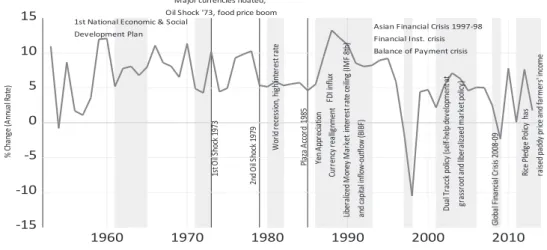
The economic growth episode of Thailand has taken-off since 1954 and continually expanded until 1960. Investment promotion policy had been the main thrust of the first National Economic and Social Development Plan. Under the plan, basic institutions were set up to facilitate planning and infrastructure development. Growth was interrupted after 1973 where major world currencies were floated and commodities boom flowed by the first oil crisis in 1973. Thailand was still benefited from this price hike as her agriculture prices were also lifted. She was truly affected by the second oil crisis in 1979. This time Thailand was suffered from a world recession after a high-interest rate thereby slow down world demand for Thai export and slowdown the domestic economy. Growth performance was quite moderate with 5 percent per year lower than her potential growth.
-15 -10 -5 0 5 10 15
1960 1970 1980 1990 2000 2010
% Ch an ge (A nn ua lR at e)
Major currencies floated, Oil Shock '73, food price boom 1st National Economic & Social
Development Plan
1s tO ilS ho ck 19 73 2n dO ilS ho ck 19 79 Pla za Ac co rd 19 85 Ye nA pp re cia tio n
W or ld re ce ss ion ,h igh int er es tr at e Cu rr en cy re all ign m en t FD Iin flu x Lib er ali ze dM on ey M ar ke ti nt er es tr at ec eil ing (IM F8 th ) an dc ap ita lin flo w- ou tfl ow (B IB F)
Asian Financial Crisis 1997-98 Financial Inst. crisis Balance of Payment crisis
Du al Tr ac ck po lic y( se lf- he lp de ve lop m en ta t gr as sr oo ta nd lib er ali za ed m ar ke tp oli cy ) Ric eP led ge Po lic y ha s ra ise dp ad dy pr ice an df ar m er s' inc om e
Gl ob al Fin an cia lC ris is 20 08 -0 9
Economic Chronology of Thailand 1960-2014
Figure 1: Economic Chronology of Thailand 1960-2014
Figure 1: Economic Chronology of Thailand 1960-2014
Note: The economic chronology has not described the domestic disruptions from a series of political unrests in Thailand. We have treated them as endogenous impulse responses to external shocks e.g., Vietnam War and between imbalanced class struggles among the power bases. It is assumed to be non-economic Chronology as such.
The world’s major developed countries led by the US had agreed with Japan to realign ‘Yen’ to its real value. The Japanese currency was appreciated from 220 Yen per US dollar to a much stronger position after the ‘Plaza Accord’ in 1985. This has led the Japanese foreign direct investment poured to other East and Southeast Asian courtiers. Thailand was one of the major recipients of FDI from Japan and other developed countries during the 1987-1990’s. Thailand had an imbalance of the ‘saving-investment’
therefore decided to liberalize the money market to comply with IMF 8 th article. This was to free the ceiling of interest rate, allowing a free flow of foreign capital under the ‘Bangkok International Banking Facility’ or BIBF scheme.
The liberalization of the money and the capital market had violated the open economy macroeconomic constraint. It is named the ‘Impossibility Trinity’ where the fixed exchange rate regime is operated to stabilized export earnings but allowing for free capital flow. The interest rate arbitrage would need to run a high-interest policy domestically. This will harm export as the cost of production of export will increase. Thus, the free capital inflow would be required to cushion the rising of domestic interest rates.
The cheap capital and oversupply of money have caused any inflationary impact. To hedge against these inflationary, speculators would need to hoard non-producing assets rather than real investment goods.
This had resulted in the accumulation of ‘non-tradable’ goods such as ʻreal estate’. Land price has
boomed artificially. It helped to dress up the balance sheet of private banks and finance companies. The
Asian Financial Crisis (AFC) had originated from Thailand in 1997, as the bubble busted, banking
crisis, and balance of payment crisis thereafter. The Bank of Thailand was defeated by currency
speculators or hedged funds in the currency war in February and May 1997.
The government after the AFC had managed to pay back the ‘rescue funds’ of 17.4 billion US dollars arrangement under the IMF’s balance of payment facilities. Thai currency was stabilized though much weaker than the pre-crisis level. The weak currency after the crisis had stimulated an export expansion in the world commodities market. The introduction of the ʻdual-track’ policy by the subsequent government has introduced a self-help or grass-root development in juxtaposition with market-driven policy and deregulations. The Thai economy had recovered and ready to take-off to another growth episode of competitiveness in outward-oriented export earning policy. Thai economy was not severely affected by the Global Financial Crisis in 2008-2009. The economy was further stimulated by the ‘Rice Pledge’ policy which had raised the paddy price and farmer’s income.
In short, Thailand started her economic development during 1950-1960 with growth in agriculture. It was dominated by primary products like paddy, timber, and tin, etc, for export earnings. During1970’s she has earned foreign currency from four main cash crops like paddy, cassava, maize, sugar cane, and natural rubber. In the 1980s, Thailand has taken off to light industrialization in food production and others. After the ‘Plaza Accord’ and Japanese Yen appreciations after 1985, Thailand had received an influx of foreign direct investment from Japan and East Asian countries. This may be the beginning of light industrialization with labor-intensive and later shifting to capital deepening in her industries in the late 1990s.
2.1 Sources of Growth in Thailand
Ketsawa (2019) 4 has pointed out that the domestic demand expansion mainly determined the sources of industrial growth in Thailand from the demand side as compared with export expansion and import substitution. The electronic and electrical machinery, transport equipment, rubber and plastic, and textile had contributed to manufacturing growth in Thailand. The growth of gross output of these industries was 17.4, 13, 9.4, and 8.6 percent, respectively. The transport equipment, chemical, electrical machinery, and other capital-intensive industries had their domestic demand and export as significant sources of industrial growth. Also, the industries had significant backward linkage.
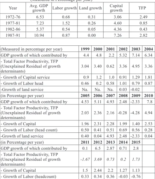
The analysis of the sources of growth from the supply-side has found that the growth of real GDP was contributed by the growth of capital and labor inputs weighted by their value-share or factors’ prices and technology. The growth’s residual unaccounted by capital and labor in the growth accounting is nominated as the growth of technology. It is called ʻTotal Factor Productivity’. Applying the ‘growth accounting’ 5 of Thailand, we have found that TFP growth was quite impressive during 1972-1991, 1999- 2004, it may mean that TFP has contributed in line with human capital and physical capital growth contribution.
It was hypothesized that the TFP may have been higher if the capital deepening process exhibited higher productivity and efficiency. It was criticized by Krugman 6 “if growth in East Asia has been primarily input-driven, and if the capital piling up there is beginning to yield diminishing returns. ...
and there is no sign of such exceptional efficiency growth.” Thus, the ‘East Asian Growth Miracle’
including Thailand was heavily reliant on the growth of capital input. Moreover, it may mean that Thailand may have over-invested in capital deepening. That is, Thailand did not have a ‘quality growth’
with high TFP.
4
Ketsawa, W. (2019) “Industrial Growth and Development in Thailand 1980-2010: A Lesson Learned for CLMV”, The Social Science Review: Special Issue on Mekong Economy, No.156 March 2019, pp.51-70
5
GDP growth per year ln(Y) = [growth of capital input ln(K)*value share of capital (r*K/Y)] + [growth of Labor input ln(L)* value share of labor (w*L/Y )] + [growth of land services ln(Land)*value share of land (rent*Land/Y)] + Total Factor Productivity
6
Krugman, P. (1994), Ibid. a quotation is from his paper on pages 11-12.
See also World Bank (1993), The East Asian Miracle: Economic Growth and Public Policy, Oxford University Press http://
documents.worldbank.org/curated/en/975081468244550798/pdf/multi-page.pdf accessed May 25, 2019.
Table 1: Sources of Growth from the Supply Side in Thailand 1972-1991 (Measured in Percentage per year)
Year Avg. GDP
growth Labor growth Land growth Capital
growth TFP
1972-76 6.53 0.68 0.31 3.06 2.49
1977-81 7.23 1.52 0.26 4.60 0.85
1982-86 5.37 0.54 0.05 4.36 0.43
1987-91 10.94 0.87 0.00 7.26 2.82
(Measured in percentage per year) 1999 2000 2001 2002 2003 2004 GDP growth of which contributed by 4.4 4.8 2.2 5.32 7.14 6.34 - Total Factor Productivity, TFP
(Unexplained Residual of growth
determinants) 3.04 3.40 0.62 3.36 4.95 3.36
- Growth of Capital service 0.9 1.2 1.0 0.91 1.29 1.81 - Growth of Labor head 0.46 0.2 0.58 1.01 0.79 0.87 -Growth of land service Na. Na. Na. 0.03 -0.02 (in Percentage per year) 2005 2006 2007 2008 2009 2010 GDP growth of which contributed by 4.53 5.11 4.93 2.48 -2.33 7.8 - Total Factor Productivity, TFP
(Unexplained Residual of growth
determinants) 2.03 2.36 2.16 -0.28 -4.28 4.94
- Growth of Capital 1.96 2.31 2.28 1.99 1.40 2.53 - Growth of Labor (head count) 0.50 0.41 0.51 0.69 0.56 0.28 -Growth of land service 0.40 0.04 4.93 2.48 -2.33 0.04 (in Percentage per year) 2011 2012 2013 2014 2015 GDP growth of which contributed by 0.1 6.5 2.87 0.71 2.8 - Total Factor Productivity, TFP
(Unexplained Residual of growth
determinants) -1.67 3.69 0.73 0.2 1.73
- Growth of Capital 1.5 2.44 2.2 1.27 1.13
- Growth of Labor (headcount) 0.33 0.34 0.36 -0.03 -0.76
Note: real GDP, labor land, and Capital and TFP expressed in terms of percentage change per year.
Source: NESDB and own calculations
We have not estimated the sources of growth owing to human capital growth in our paper. If this is taken into account, the sources of growth may be somewhat changed on the labor headcount to be lower and replaced by the growth contribution from the human capital. The integration between growth contributions from the demand-supply side should be interpreted as follows: Firstly, the influx of foreign direct investment during 1987-1997 had given rise to rapid expansion on the demand side as had been pointed by Ketzawa (2019) 7 . Thus, the process of capital deepening applying low-wage labor in Thai manufacturing sectors was sources of growth from the supply side as well. This was pointed by Bowonthumrongchai (2019) 8 that Thailand has passed the ʻturning point’ of several criteria proposed by
7
See Ketsawa, W. (2019) Ibid.,
8
Bowonthumrongchai, T. (2019) “Economic Development and Urbanization in Thailand 1960-2015: Implication for the Mekong”,
The Social Science Review: Special Issue on Mekong Economy, ???..
Minami (1968) 9 . Thus, there was an internal migration of unskilled labor with low-wage from the rural area (agriculture sector) to the urban area (manufacturing sector) in the Thai context. The capital deepening by the manufacturing and service sector without a proper plan for skills formation on the human resource had caused overcapitalization without matched skills. In an economic term, it may be described as unsustainable capital intensity (capital-labor ratio) growth path. The immediate response was a decline in profit rates of heavy industries as compared with light industries in the capital market.
It was Krugman (1994) 10 who firstly observed and warned about over capital accumulations in Thailand and other East Asian countries. Capital utilization was not efficient and may face diminishing returns.
The macro-economic policy during 1994-1997 has proved to be imprudent as Thailand has complied with the IMF suggestion on the liberalization of the interest rates while allowing the free flow of foreign capital under the Bangkok International Banking Facilities. The declining rate of profit in the real sector has motivated investors and private funds to shift to invest in the non-performing loans i.e., real estates and non-tradable activities rather than R&D capital investment and human skills development.
After the AFC in 1997-1998, the foreclosure of non-performing financial assets had caused a decline in the physical capital of the real sector. Especially, the enterprises with Thai capitals were tragically declared bankruptcy and changing ownerships. Now the economic development of Thailand has turned into an episode of low-level capital accumulation opposite to what has happened before the AFC. Most of the private financial institutions were majorly owned by foreign capital. They were prudential on project loans for most of the firms. Thai firms had a hard time raising capital from the secondary capital market and debt market to finance their capital investment as well. Therefore, Thai firms in light industries and services, etc. that utilized labor-intensive, unskilled labor would seek to hire foreign guest laborers to reduce their production cost. The suppression of low-wage unskilled workers had prolonged the resumption of capital investment in most of the labor-intensive sectors. An exception may be only the foreign firms with their own capital could still make a capital investment. But, actual growth performance was lower than the potential growth after AFC 1997 until at least 2010. Capital dilution which was an opposite scenario of capital deepening was phenomena in Thailand after 2000 until the current date of 2020.
3. Review of Theoretical Models
We visualize that Thailand has been developed through stages of the ‘Indicative Planning Model’
drawn by the National Economic and Social Development Board, the Thai government. The National Economic and Social Development Plans since the early 1960s until now are altogether 12 plans. Most governments either elected under a democratic system and/or non-elected governments have mostly followed these indicative plans. Some democratic government has set her execution agendas according to these plans plus their own campaigned agendas. Thus, we may imagine that the execution agenda of each government was different in degree of dependency between indicative planning vis-à-vis market- oriented mechanism liberalization. It is postulated that Thailand may have applied some kind of planning process since the 1970s.
3.1 The Ramsey Model 11
Ramsey firstly asked the question of ʻhow much of income should a nation save?’. He tried to apply the mathematical model to solve this puzzle. Ramsey’s postulated that ʻThe rate of saving multiplied by the marginal utility of money should always be equal to the amount by which the total net rate of enjoyment of utility falls short of the maximum possible rate of enjoyment.’ 12 Ramsey described the maximum obtainable rate of enjoyment or utility and called it, for short, the ʻBliss’ which the community must save enough either to reach Bliss after a ‘finite time’, or at least to approximate to it indefinitely.
9
Minami R. (1968) “The Turning Point in the Japanese Economy”, The Quarterly Journal of Economics, Volume 82, Issue 3, 1 August 1968, pages 380-402.
10
Krugman, P. (1994), Ibid.,
11
Ramsey F.P. (1928), “A Mathematical Theory of Saving”, The Economic Journal, Vol. 38, No. 152 (Dec. 1928), pp. 543-559, Published by Blackwell Publishing for the Royal Economic Society, Stable URL: http://www.jstor.org/stable/2224098, Accessed:
09/12/2010 04:55
12
Italic is Ramsey’s original, p 543.
Ramsey firstly started from the simple account identity that the savings plus consumption must equal income. Then, he defined the marginal rate of utility as a function of the frequency of consumption flow and the disutility of a rate of labor supply flow. The difference between the total rate of utility and disutility is ʻnet enjoyment’ which is subjected to a given level of capital stock. The planner would aim to maximize net enjoyment over time. The maximal conceivable limit of net enjoyment is reached without further increase in either income or leisure by an increment of capital. He called it the ʻmaximum obtainable rate of enjoyment’ or ʻBLISS’ which strictly reach only at the limit. The more the nation
‘save’ (sacrifice of the enjoyment we have now) the feasible it can approach the bliss earlier. Ramsey has proved that the ʻrate of saving multiplied by the marginal utility of consumption should always equal bliss minus the actual rate of utility enjoyed’ 13
Ramsey model differed from the Solow-Swan model 14 in crucial assumption on the saving rate. In Solow-Swan, the fraction of output is saved at a constant rate s, so that the saving is sY(t). Solow assumes the production function is homogeneous of the first degree (leads to a constant return to scale of factors), thus, no scarce non-augmentable resource like the land that would lead to decreasing returns to scale in capital and labor and the model. The growth of the labor force was exogenously given, as long as real income was positive, the positive net capital formation must result. If savings fall to zero when income is positive, it becomes possible for net investment to cease.
Ramsey growth model was extended by Cass and Koopmans such that households explicitly optimize the choice of consumption at a point in time. Thus, the model has an endogenous savings rate as a variable saving rate along with the transition to the long-run steady state. It is also a Pareto optimal.
Unlike the originally Ramsey which is a central planner’s maximizing levels of consumption over successive generations, Cass and Koopmans’s model describes a decentralized dynamic economy explaining long-run economic growth.
In a developing country like Thailand, it has been perturbed by the business cycle fluctuations with market imperfections and heterogeneity among households. It is interesting if the role of the government is considered as well.
3.2 The Indicative Planning Model à la Ramsey-Cass-Koopmans (RCK)
The production function is neoclassical Cobb-Douglas technology, Y=K α L 1-α ; 0<α<1, or y=k α shown in per-capita terms. We omit technological progress in accordant with the stylized fact mentioned for Thailand and assume the population growth at a constant rate. The utility function is assumed as u(c)= c 1-σ
1-σwhere σ> 0, the social welfare optimization is subjected to the economies’ resource constraint given by =y-c-(n+δ)k. The change in the capital (physical and human) is equal to the saving (y-c) minus by the depreciation plus population growth rates (n+δ), all are in terms of per capita.
The social planner objective is to maximize welfare measured by the following:
(1) (2) The current-value Hamiltonian
(3)
λ is the co-state variable, c is the control variable, and k is the state variable.
13
Italic is Ramsey’s original, p 547.
14
Solow, Robert M. (1956). “A contribution to the theory of economic growth”, The Quarterly Journal of Economics, Vol. 70, No.
1 (Feb. 1956), pp. 65-94, The MIT Press, doi:10.2307/1884513. Stable URL: http://www.jstor.org/stable/1884513. Swan, Trevor
W. (November 1956). “Economic growth and capital accumulation” Economic Record. 32 (2): 334-361. doi:10.1111/j.1475-
4932.1956.tb00434.x.
The first-order conditions are given by
(4) (5)
(6) The transversality condition
(7) From (4), take a log and differentiating with respect to time yields
Re-arrange (6), yields (8)
(9)
From (8) and (9) together, we get the Keynes-Ramsey rule. The equilibrium has saddle point property as can be observed in the usual phase diagram. By the Hartman–Grobman theorem the non-linear system is topologically equivalent to a linearization of the system about ( , ) by a first-order Taylor polynomial
(10) (11) (12)
The transversality condition ensures convergence towards the interior steady state. The steady-state values are
(13) (14)
At steady state, the Jacobian matrix of the RCK 15 is
become
has its determinant .
Since c is always positive and σ is positive by assumption, the only ( ) is negative since is concave.
The determinant has one eigenvalue greater than zero and the other is opposite in sign.
Besides, it is assumed that the inefficient over saving (non-Ponzi game or ) cannot occur in the optimizing framework. Thus, the equilibrium is a saddle point and there exists a unique stable arm or saddle path that converges on the equilibrium. The saddle path is stable or not depending on the property of the economic structure and the nature of the external shocks.
In Thailand, the government had implicitly followed these indicative planning rules which could work efficiently with the market mechanism. The RCK model with the government in a normal market economy is simply explained as follows:
The government has introduced proportional taxes on wage w,τ w ; on the private return on asset a, τ a ; and on the private consumption c, τ c respectively. Thus the representative household’s maximization problem is now simply to
15
Matrix of the partial derivatives of (10) and (11) with respect to (k,c).
(15) (16)
whereas c denotes consumption per-capita, k the capital stock per-capita, T lump-sum transfers, w the wage rate, r the interest rate, σ the inverse of the intertemporal elasticity of substitution, and ρ the discount factor, respectively. The government is assumed to run a balanced budget. It means government revenue will be spent back to the economy via lump-sum transfer to households. The production function is neoclassical Cobb-Douglas technology
(17)
where, Y denotes the output, K the capital stock, L the amount of labor employed in production, and α the elasticity of capital in the final output production, respectively. Since perfect competition in factor markets is assumed, firms pay the factors according to their marginal product,
(18) (19) Solving the household’s optimization problem yields the Keynes-Ramsey rule
Assuming capital market equilibrium k yields the system
(20) (21)
with initial condition k (0) = k0 equation (18) and (19) can be inserted into the system (20) and (21), or treated as algebraic equations for the numerical simulation. It should be noted that the optimal economic growth has been extended to incorporate the fiscal-monetary policy in an aggregative form by Uzawa H.(1998) 16 . The study has applied an exogenous income tax rate and growth rate of money supply such that an optimum rate of investment is attained through time. The economy produced public goods and private goods respectively. The former is regarded as consumption goods by Uzawa while private goods can either be consumed instantaneously or accumulated as capital. The study has explicit social welfare function which is defined as the discounted sum of the instantaneous utilities through time. It is however interesting that Uzawa has reformulated the problem of fiscal policy such that the public sector seeks optimal time-paths of factor and output allocations by choosing appropriate dynamic fiscal policy parameters i.e., tax rate and increases the rate of the money supply 17 . Cass (1965) 18 proved the optimal growth model applying the calculus of variation and the ‘Maximum Principle’. Cass acknowledged Koopmans (1963) 19 who arrived at the same conclusion on the ‘Keynes-Ramsey’ rule with ‘bliss’ replaced by golden rule of individual welfare. Furthermore, Cass noted that the limiting optimum path is similar to those found by Srinivasan (1964) 20 and Uzawa (1964) 21 . However, they both assume that the utility index is simply consumption per capita, while in Cass’s model he introduced a diminishing marginal rate
16
Uzawa, H. (1988), “Optimum fiscal policy in an aggregative model of economic growth”, Chapter 18 of Preference Production, and Capital: Selected Papers of Hirofumi Uzawa_Cambridge University Press, pp.313-39
17
See Uzawa, H (1988) p.338.
18
Cass, D. (1965), “Optimum Growth in an Aggregate Model of Capital Accumulation”, Review of Economic Studies No.32, pp. 233-240.
19
Koopmans T.C. (1963), “On the Concept of Optimal Economic Growth”, Cowles Foundation Discussion Paper, December.
20
Srinivasan, T. N. (1964), “Optimal Savings in a Two-Sector Model of Growth”, Econometrica, No. 32 (1964), pp. 358-373.
21
Uzawa, H. (1964), “Optimal Growth in a Two-Sector Model of Capital Accumulation”, Review of Economic Studies, 31 (1964),
pp. 1-25.
of substitution between generations’ welfare. Ohdoi R. (2016) 22 has incorporated government intervention into the baseline RCK model. It is proved that the government spending crowds out private consumption.
The consumption tax’s distortion is less as long as the same rate applies to all goods and it is constant over time. Moreover, capital income taxation harms the households’ savings, thereby capital accumulation. In consequence, the capital stock in the steady-state decreases as the tax rate becomes higher. By introducing the labor-augmenting technological change to the baseline model, all per capita variables (per capita GDP, capital, consumption...) become to grow at the same constant rate of technological progress in the long-run.
3.3 Debate on the Choice of Capital Accumulation
Inada, Sekiguchi, and Shoda (1992) 23 analyzed capitalization along the growth path of the ‘Three- Sector model of economic growth’. The literature has drawn heavily to prove the growth of lower capital intensity towards the higher capital intensity sector empirically. The movement of low to high capital intensity is quite interesting and maybe point of discussion to explain the situation of contemporary Thailand ‘why’ we are not able to get out of the ‘middle-income trap’. Inada’s three-sector model had built up an ex post-theoretical model to explain how the economy e.g., pre modern-Japan which had limited resources allocate [capital] to nurture her industrialization away from the subsistence sector (the S-sector), passing the light industry sector (the X-sector), to the heavy and chemical industry sector (the Z-sector). The characteristic of S-sector is the same as Lewis 24 , ʻdisguised unemployment’ and being the main supplier of low-wage labor to the X and Z-sector respectively. Noting in the case of Thailand, Bowonthumrongchai (2019) 25 has proved that Thailand has passed over a ʻturning pointʼ using several criteria proposed by Minami (1968) 26 .
The main hypothesis of Inada’s ‘three-sector model’ are (1) if the amount of accumulated capital in the X-sector increases, the profit rate of the sector (R X ) declines, exhibiting constant return to scale of production and (2) As the Z-sector has increasing return to scale of production if the amount of accumulated capital in the Z-sector increases, its profit rate (R Z ) rises. It is assumed that the wage incomes in the S-, X-, and Z-sectors are spent entirely on consumption. The sum of investment in the X- and Z-sectors is equal to the sum of profits in the X- and Z-sectors. Thus, firms will optimally allocate their retained profit to invest in a sector that is the most profitable between X- and Z- sector. The Inada’s model was a replica of what has been achieved in Japan and East Asian countries, in the early days of development. The model can be extended to cope with the open economy to have net capital inflow from abroad in terms of foreign aid (ODA). The model has its fundamental belief that heavy government intervention i.e., high import tariff to protect domestic infant industries, import of technology, heavy subsidy to the Z-sector would be sufficient conditions to take-off. This may or may not be true for most developing countries to replicate Japan.
The foregoing postulation is based on the neoclassical tradition. Especially, the smooth production functions with continuous substitution pioneered by von Neumann (1945-1946) 27 and Dorfman, Samuelson, and Solow (1958) 28 , Morishima (1964) 29 respectively. Even though, Neuman had started with the finite array of linear technologies rather than continuous substitution and related core issues. It was later related to the issues of the factor price frontier, re-switching of production techniques by
22
Ryoji Ohdoi (2016), Ramsey-Cass-Koopmans Model (1) and (2) lecture notes, based on Acemoglu (2009), Blanchard and Fischer (1989) and Barro and Sala-i Martin (2004), Dept. of Industrial Engineering and Economics, Tokyo Tech. https://www.google.
com/search
23
Inada k., Sekiguchi, S. and Shoda, Y (1993), Mechanism of Economic Development: Growth in the Japanese and East Asian Economies. Oxford and New York: Clarendon Press, I993.
24
W A (1954) “Economic Development with Unlimited Supplies of Labor”, Manchester School of Economic and Social Studies, Vol. 22, pp. 139-91.
25
Bowonthumrongchai, T. (2019), “Economic Development and Urbanization in Thailand 1960-2015: Implication for the Mekong”, The Social Science Review: Special Issue on Mekong Economy, ???..
26
Minami R. (1968) “The Turning Point in the Japanese Economy”, The Quarterly Journal of Economics, Volume 82, Issue 3, 1 August 1968, pp. 380-402.
27
Von Neuman, John. (1945-46), “A Model of General Economic Equilibrium”, Reviews of Economic Studies, Vol. 13, pp. 1-9.
28
Dorfman, R., Samuelson, P. A., and Solow, R.M. (1958), Linear Programming and Economic Analysis, New York, McGraw-Hill.
29
Morishima, M. (1964), Equilibrium Stability and Growth: A Multi-Sectoral Analysis, Oxford University Press.
(Pasinetti, and others) 30 . It further leads to the debate between Classics, Post-Keynesian, and Neo- classical economists as noted by Marglin (1984, p.540) 31 on multiple technologies and the re-switching.
ʻReswitching was held to be important…..it is sufficient but not necessary condition…..the failure of the monotonicity in the correspondence between the capital intensity of production and the rate of profit….be understood as part of …the larger debate….about the existence of the “well-behaved”
capital aggregation in the multiple-good world.’
Burmeister and Dobell (1970) 32 have applied Leontief model with Technique α and the corresponding
matrix of input coefficient vector where and , (i=1,2,…,n;
j=0,1,…,n) where L j , K j , Y j is labor, capital inputs and output respectively. Given W(t)=[W 0 (t),W 1 (t),...,W n (t)] where W 0 (t) is the nominal wage rate paid at the end of the period t and W i (t) the gross rental rate for the i-th capital good paid at the end of period t. They defined the equilibrium price with one technique matrix as P(t+1)= a 0 W 0 (t)+P(t)ρ(t)a where P i (t) ,(i=0,1,,…,n) the price of one unit of the i-th output at the beginning of period t and P(t)=[P 0 (t),P 1 (t),….,P n (t)].
They noted on page 231 further that W i (t)/P i (t)≡ρ i (t)= the gross own-rate of return for the i–th capital goods, (i=1,,…,n) and the net own-rate of return for the i-th good r i (t) ≡ρ i -δ i where δ i is depreciation rate and r 0 (t) = the money rate of interest or the profit rate. [ θ+δ ] is a diagonal matrix with (1,θ+δ 1 ,….,θ+δ n ) and [ ρ ] is the diagonal matrix with (1,ρ 1 ,….,ρ n ) on the diagonal and [0] on the off-diagonal row-column. Hence, in matrix notation p = a 0 + pρa where p≡ ( ) and p=
a 0 [I- ρa] -1 where ρ is own-rate of return for the i-th capital good. If matrix p>>0 is strictly positive, the net own-rate of return for the i-th capital good r i satisfy r i =0 for i=1,…,n. The scalar r 0 is called a feasible rate if the matrix ρ is feasible when r i = r 0 ,i=1,…,n. Then it is proved ≥0, (i=0,1,2,…,n;
j=1,…,n) if the j-th capital good is required, directly or indirectly for the production of good i. This implies a non-negative relationship between gross own-rate of return and price of output.
Burmeister and Dobell (1970) generalized his proof to an alternative set of technique matrices S_technique ≡ {α,β,…η,…|the given ρ is feasible} such that the equilibrium prices p i (η), i=1,…,n, satisfy the inequality p(η)≤ a 0 (.)+p(η)ρa(.) where a(.) is a convex combination of technique matrices belong to S. Equilibrium prices are functions of exogenous profit or interest rate r 0 . If r i (t) ≡ρ i -δ i = r 0
=0 for example then technique α is employed, it is feasible if and only if r 0 <1/ ≡ (α) where is the dominant characteristic root of the matrix a(α)[I- δa(α)] -1 .
The survey above gives the meaning for our study as follows: 1) The factor-price curve (FPC) where a horizontal axis of the interest rate or profit rate r 0 the plot against real wage ≡ for Technique α that belongs to the set S_technique is downward sloping. 2) With several techniques in S the FPC are downward sloping but can have any shape since their sign of the second derivative is ambiguous.
However, their outer envelope or the economy’s FPC can be derived. 3) The ‘re-switching’ implies an entire technique in S_technique recurs at a different profit or interest rates. This proof is to counter non- neoclassic tradition especially Sraffa (1960) and Passinetti (1966) 33 that it is contradicting or paradoxical or perverse to the neoclassical setting. Burmesiter and Dobell (1970) further responded that it is can occur even if the alternative technique matrices are all indecomposable. 4) They have finally proved that the re-switching of technique may occur but only sufficient but not necessary. It is impossible in the neoclassical multi-sector model without joint production 34 .
30
Pasinetti, Luigi L.(1966), “Changes in the Rate of Profit and Switches of Technique”, The Quarterly Journal of Economics, pp.503-17; Sameulson, P., Modigliani (1966), “The Pasinetti Paradox in Neoclassical and More General Model”, Review of Economic Studies, Vol.33, pp. 269-301; Morishima, M. (1966), “Refutation of the nonswitching theorem”, Quarterly Journal of Economics, vol. 80, pp.520-525; The debate followed the pioneer paper by Sraffa, P. (1960), Production of Commodities by Means of Commodities: Prelude to the Critique of Economic Theory, Cambridge University Press.
31
Marglin S., A. (1984), Growth, Distribution, and Prices, Harvard University Press.
32
Burmeister, E. and Dobell A., R. (1970), “Leontief Models with Alternative Technique”, Chapter 8 of Mathematical Theories of Economic Growth, Macmillan Publishing Co., Inc. New York., pp. 228-271
33
See Sraffa (1960), Ibid.; Passinetti (1966), Ibid.; and Marglin S., A. (1984), Ibid.; See more detail in next section.
34
Burmeister and Dobell (1970), See Theorem 5 page 297. ibid.; Burmeister, E. (1980), Capital Theory and Dynamics Cambridge
Survey of Economic Literature, Cambridge University Press.
In dynamic Leontief models, Taylor (1979) 35 pointed out the role of investment and capital accumulation, let b ji = K ji /X i be capital-output ratio. Assuming that there is no substitution among capital types and some sectors only produce capital goods, the rest of the sectors have b ji =0. If the economy is working at full capacity, then any increment in production is supported by new capital stock in place next year. The material balance equation is thus
and in matrix notation X(t)= AX(t) + B[X(t+1)-X(t)]+ F(t). If the economy grows at a constant rate . Then the homogenous equation (I-A-gB)X(t)=0 with no consumption when exogenous final demand F(t)=0. Then maximal growth of this economy is possible when surplus products are being invested. The maximal growth rate can be determined from the determinant applying the Perron 36 a theorem that B(I-A) -1 are nonnegative. There will be a positive growth rate with corresponding positive eigenvector at which steady growth is possible. The corresponds to the largest (1/ ) that solves the above determinant. Investment demand in an open economy I-O may be related to capacity increments rather than output as X(t)+ M(t)=
AX(t) + B[CAP(t+1)-CAP(t)]+F(t); with a restriction on X(t)<<CAP(t); and M(t)[CAP(t+1)-X(t)]=0 where M(t) is import matrix (non-competitive type) which implying production in each sector cannot exceed its capacity and the competitive import is positive only if capacity is fully utilized to close the gap. Along the balanced growth path, all sectors are expanding at the same rate. The output vectors , satisfy the optimal growth path of output as primal solution while Sraffa’s prices satisfy the optimal growth path of the price as a dual solution.
According to Taylor (1979, p. 192), the author relaxes the assumption on final demand F(t)>0 grows at a rate of h under the growth path of a dynamic system X(t)= (I-A-hB) -1 F(t) as long as the rate . The aggregate saving rate and the capital-output ratio at Sraffa’s prices can be determined as
follows: Let Z T =[1,1,….,1] and savings rate s = and =
= along the steady-state growth path. We observe Z T (I-A*) X*-Z T X*=hZ T B*X* on the output side and P Sraffa T (I-A)X-P Sraffa T F=hP Sraffa T BX on the cost per unit or price side so that saving equal investment.
We do not involve in such a debate between eminent economists in the last decades. What we are interested in is that what will be the behavior of correspondence between the capital intensity of production and the rate of profit, the factor-price frontier, the well-behaved production function, etc., in the case of Thailand during economic development. We wonder that the factor-price frontier of the production system exhibits a well-behaved manner or not. In short, is it possible that the capital deepening before the AFC was not well-behaved? The pre-AFC was deepening with an overcapitalization such that the slope of the FPC has perverse sign reflecting in an upward sloping demand for factor inputs i.e., the higher profit rate is perversely correspondent with higher capital-labor ratio, More importantly, we would like to know whether the real wage-profit rate or the factor price curve are well-behaved as a conjecture by the neoclassical model.
On the contrary, after AFC in 1977, capital accumulation was much under the sustainable level for the potential growth of the Thai economy. The production system in Thailand has chosen to bundle unskilled labor with cheap wages rather than to accumulate new capital with higher technology. The factor price frontier between profit rates and real wages may have another feature. In our paper, we have constructed the constant price dynamic I-O Tables of Thailand 1975-2010. We will explore the numerical evidence of these puzzles.
3.4 Growth and Income Distribution: Post Keynesian Approach
Luigi L. Pasinetti is an eminent economist of the post-Keynesian school the heir of the “Cambridge Keynesians” and a student of Sraffa and Kahn. He has also developed the theory of structural change and
35
Taylor, L. (1979), Chapter 12 The dynamic Input-Output model and the Sraffa’s price, in Macro Models for Developing Countries, Economics Handbook Series, McGraw-Hill Book Company.
36
The singular matrix with 0 determinant, all element of I-O matrix A are non-negative such that each sector requires inputs from
every other sector at least indirectly, the polynomial equation in will have positive root (Eigen root) larger in magnitude than any
other Eigen value.
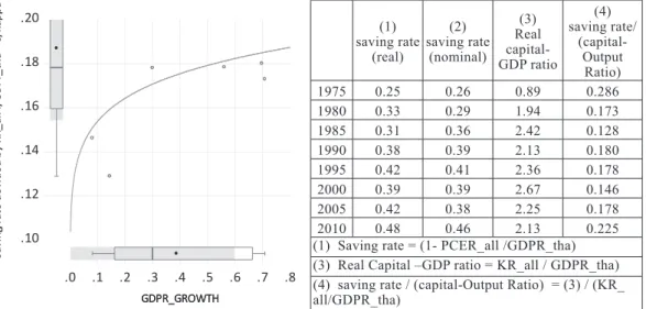
economic growth, structural economic dynamics and uneven sectoral development. Following Pasinetti (1974, Chapter IV) 37 section 5 on ‘Long-run equilibrium conditions by Domar (1946) 38 as follows: Given the investment, influences total effective demand (1/s) I = Y, through (1/κ) I = CAP/dt , where I= new investment, CAP = productive capacity, κ= capital-output ratio, Y= net national income, s = savings to income ratio respectively. The equilibrium between effective demands Y may not necessarily guarantee the full capacity utilization CAP. Domar illustrated that given the initial condition where CAP (0) = Y (0) at time=0. Then if the productive capacity over time (dCAP/dt) = (dY/dt) the effective demand, after substitution, we obtain (1/κ) I= (1/s) (dI/dt) from which (s/κ) dt = (1/I)dI.
By integration and the initial condition of I (t) =I (0) e (s/κ) . The ʻe’ is the exponential rate, or the percentage rate of growth per period considered and the investments must expand at a percentage rate of growth g equal to s/κ or the ʻwarranted rate of growth’ g = . Harrod (1948) 39 defined it as the rate of growth at which the producers will be content with what they are doing. This can happen when net income, consumption, and the stock of capital will all grow at the same percentage rate g. The equilibrium may be violated in the long-run where full capacity utilization may not guarantee the ‘full employment’.
Harrod’s contribution to the ʻnatural rate of growth’ may fill this gap. Given the labor force growth L(t)=L(0)e (nt) and average productivity of labor y(t)= y(0)e (λt) where L(t)=labor force at time t, and n = percentage rate of growth of labor force, y(t)= Y(t)/L(t) and λ = percentage rate of growth of productivity.
Thus, g n =n +λ is the ‘natural rate of growth’. It is the maximum sustainable growth rate that technical condition makes available to the economic system as a whole. Then full employment of labor force and full utilization of productive capacity take place only if the natural rate of growth and warranted rate of growth equal or g n = g and thus s = κg n the saving ratio (s) must be equal to the capital-output ratio multiplied by the natural rate of growth if equilibrium with full employment and full capacity utilization is maintained in the long run. The growth of investment emerges as a solution to keep full employment and full capacity utilization.
Pasinetti (1974) has further corrected the assumption of the Harrod-Domar model that treats s, κ, g n
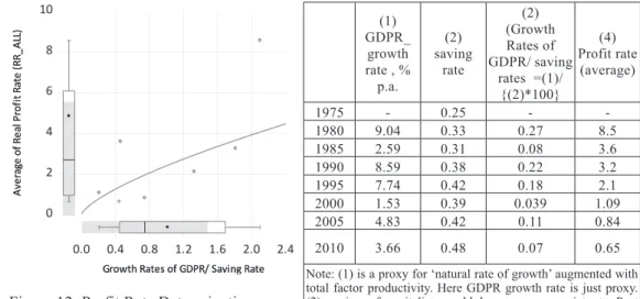
as constant and making the equality between s=κg n which is not always guaranteed. One parameter must be treated as a variable. This leads to the determination of the rate of profit and income distribution to the rate of profit and economic growth 40 . The model starts with identity P≡ P c + P w where P c , P w are profit which accrued to capitalists and workers respectively. The Equilibrium condition between investment and saving is therefore: I = s w (W+P w ) +s c P c = s w Y + (s c –s w ) P c and
and and and Finally, P/K = (1/s c ) (I/K) and P/Y = (1/
s c ) (I/Y). It means that in the long run, the propensity to save influences the distribution of income of capitalists and workers. Given a neo-classical type of production function Y= F(K,L) where labor force growth L(t)=L(0)e (nt) as usual, s c [F(K,L)-W] = I accordingly at steady- state =0 so that I = knL substituting into the equality between saving and investment we obtain s c [F(K,L)-W] = nL whence P/K = (n/sc). The equilibrium rate of profit is determined by the natural rate of growth divided by the capitalists’ propensity to save; independently of anything else in the model.
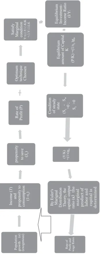
The causality chain is as follows (see figure below): the exogenously given rate of population growth and capitalists’ propensity to save determine first of all the rate of profit. At this rate of profit, the optimum technique is chosen to satisfy the marginal productivity conditions. Then the optimum technique together with the rate of population growth uniquely determines the investment-income ratio. The technical relation in the production function simply determines the equilibrium amount of capital.
Lastly, Eulerʼs theory of distribution determines the factor of income distribution between capital and labor exhaustively. The wage rate and rate of profit are determined independently from the choice of technique (shape of production function) and marginal productivities.
37
Pasinetti, L. L. (1974) Growth and Income Distribution: Essays in Economic Theory, Cambridge University Press. Chapter IV.
From Classical to Keynesian Dynamics, p.86.
38
Domar, E., D. (1946), ‘Capital Expansion, Rate of Growth and Employment,’ Econometrica, pp. 137-147.
39
Harrod, R. (1948), Towards Economic Dynamics, London.
40
Pasinetti, L. L. (1974), Ibid., p.111
According to the Keynesian view, the rate of interest has no importance in determining to save (unlike Solow Model of economic growth) but rather the propensity to consume thus propensity to save or saving rate out of income. In Pasinetti (1974, p. 127) the equilibrium relations P/K = (g n /s c ) determine the rate of profit fist of all, simply form g n (natural rate of growth) and s c (saving rate of capitalist, assuming s w =0) independent of anything else.
We would like to make another brief survey on how the factor income distribution is determined from the viewpoint of the Post Keynesian by Taylor (1979) 41 as follows:
Let X, F be a column vector of the output Xi, F i (i=1,2…N), and A the square NxN matrix. It is made up of the input-output coefficients a ij , as a result, the material- balance equation
is determined.
In compact form is X = AX + F and X= (I-A) -1 F where I is NxN identity matrix and (I-A) -1 is Leontief inverse. The cost per unit output or cost-determined output price in sector i.,
where w, r, and P 0 are the cost of labor, capital and noncompetitive imports (assumed to be equal for all sector) a Li w, a Ki r, a 0i are coefficients for labor, capital, and imports respectively.
In the base year, all prices are set to unity = 1.00. The solution (in matrix form) which implies that output price in each I-O sector is a summation of the direct and indirect primary factor costs in production.
We can view the income distribution struggle between wage earners and capitalist or between the traditional sector in the rural area e.g., agriculture with farmers – a modern sector in the urban area with entrepreneur and rentier-capitalism (landlord who control land and monopolist in the modern sector who control access to physical, financial, intellectuals, etc.,) by investigating empirically the wage- interest or wage-profit frontier.
It is the solution of the wa [I-r(I-A) -1 A] -1 X = GDP ≡ 1. The extreme case where wages=0, or wa =0 the Sraffa’s price can be found from =0; and =0. The solution of the polynomial equation in terms of 1/(1+r) associated with the 0 determinant of the matrix […] have a positive root (eigenvalue) and r max is maximal possible profit rate and positive left eigenvector in the economy P Tmax and right eigenvector or standard commodity X max respectively up to the imposition of the numeraire.
When the wage is positive scaling the employment as a X max =1 , we can obtain the income distribution as GDP=P T (I-A) X max =rP T AX max +a X max =rP T AX max +w. By rearranging we arrive at r=(1-w)/P T AX max ; AX max = (I-A)X max signifies the proportionality between intermediate and final sales of each component of the standard commodity. Finally, P T AX max = P T (I-A)X max = 1/r max . Thus, the wage-profit or wage-interest frontier in the Sraffa’s economy is r/r max = 1 – w. This implies that the wage w which is also labor share (after normalization) rises as profit rate ʻr’ falls from its maximum r max .
The Post Keynesian view is different from the Neo-classics in that the selection of production technique for all sectors, unlike Burmeister-Dobel (1970), this will lead to the highest possible r max and a set of profit maximization techniques independent of the composition of final demand. It is known as the non-substitution theorem in I-O analysis.
41
Taylor, L. (1979), Chapter 12-4 on ‘Wage and Profit Skirmishes in the Open Input-Output System’, Macro Models for Developing
Countries, Economics Handbook Series, McGraw-Hill Book Company.
Fi gu re 2 : T he Pr oce ss o f Ca pi tal A ccu m ulat io n fr om V ie w P oi nt o f t he P os t K eyn es ia n.
Popu la tion gro w th ( n ) (e xog enou s) In co m e ( Y ) an d pr op en sit y to co ns um ptio n (1 -s c )
pr open sit y to save ( S c ) Rate o f Pr of it (P) O pti m um techniqu e Choo se n
Sati sfy M ar gi nal con diti on Y=( △ Y/ △ K )K + △ Y/ △ L) L Equilib riu m Inve st m en t- Inco m e Ratio (I /Y
)Equlib riu m am ount o f Capital K (P /K) = (1/ s c )g n
C onditio n of stead y stat e (S c - S w >0 ; S c >0
(Y /K ) =(1 /s )g n
B y Eu le r's M ar ig nal D is tributi on Theo ry , the ca pital -o utput ratio ( κ) th e m ar gin al pro du ct o f lab or an d ca pit al is de ter m in ed
R ate of Pr of it an d wa ge R ate s Figure 2: The Process of Capital Accumulation from V iew Point of the Post Keynesian.
In sum, we would like to test by applying the empirical study whether the factor price curve between the profit rate and the wage rate is downward sloping in either the Neo-classic or Post Keynesian that being pointed by our survey of literature above. Besides, the relationship between the capital-labor ratio and the profit rate- wage rate and saving rate would be also another point of investigation from the dynamic I-O of Thailand 1975-2010.
4. Empirical Analysis with Open Leontief Model
We formulate the planning model to maximize welfare function over the planning period (1975- 2010). The model is subjected to constraints in the form of distribution relations, production functions, absorptive capacity functions, foreign exchange constraints, and initial and terminal capital stock and foreign debt constraints respectively. The model has four sub-sectors: (1) agriculture and mining, (2) heavy industry, (3) light industry, and (4) services. We rely on the ISIC classification under the 7 Input- Output Table of Thailand 1975-2010 respectively. We firstly estimate the capital stock which is consistent with the I-O structure in the planning period. We have applied the ‘Perpetual Inventory Method following Berlemann and Wesselhoft (2014) 42 to estimate the capital stock series.
It is assumed that the stock of inventory increases with capital formation (investments). That is the Kt =(1-δ) K t-1 +I t-1 , where δ is the geometric depreciation rate. Repeatedly substituting this equation for the capital stock at the beginning of the period, leads to the capital stock in period t is a weighted sum of the history of capital stock investments K t = (1-δ) i I t -(i+1) . Assuming the base year (origin of series) capital stock , and the depreciation rate δ the capital stock series becomes K t =(1-δ) t- 1 + (1-δ) I t-(i+1) . Berlemann and Wesselhoft have proposed the ‘Steady State Approach’ based on Harberger (1978). At the ‘steady-state’ output grows at the same rate as the capital stock
. Thus, it is sufficient to calculate the capital stock in the initial period K t-1 = . If however, there is a short-term investment shock we may have to smooth the investment series using three-year moving averages to generate stable capital stock estimates.
The study has applied the regression analysis of investments on time variables to calculate the initial capital stock. The estimation result of the imputed depreciation rate is equal to (1- 0.9652)*100 =3.48 percent per year on average for aggregate capital for national and assuming the rate for the manufacturing sector. The estimation of initial capital stock by sector for i= light industry, heavy industry K i,t-1 = with ∑ i K i,t =K t as the constraint or the summation of the capital stock of sub-sectors equal to the total capital stock in manufacturing. In short, the capital stock series are estimated from base year capital stock. 43
4.1 The Changing Trend of Economic Growth, and Productivity of Capital 1975-2010: Thailand under Asian (1997) and Global (2009) Financial Crisis
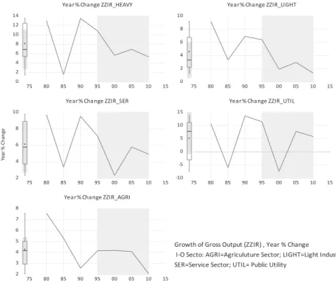
We have constructed stylized facts from the Thai I-O a 5-year interval account from 1975-2010. We have presented the related economic variables in both level form and terms of the yearly percentage change. Thai I-O was deflated with respective price indices to get a constant price I-O at 2000 prices as a basis. The graph of 5 sectors namely Agriculture, Light, Heavy, Service, and Public Utility is shown for illustration and analysis. Some aggregation is computed to arrive at the overall summary.
42
Berlemann, M. and Wesselhoft, J-E (2014), ‘Estimating Aggregate Capital Stocks Using the Perpetual Inventory Method: A Survey of Previous Implementations and New Empirical Evidence for 103 Countries ‘, Review of Economics, 65. pp. 1-34, ISSN 0948-5139.
43
Regression of (K
t-I t-1 )=f (1-δ) K t-1 , yields δ=0.035 with statistical significant P-Val=0.0, R2 = 0.99 respectively.
0 2 4 6 8 10 12 14
75 80 85 90 95 00 05 10 15
Year% Change ZZIR_HEAVY
0 2 4 6 8 10
75 80 85 90 95 00 05 10 15
Year% Change ZZIR_LIGHT
2 4 6 8 10
75 80 85 90 95 00 05 10 15
Year% Change ZZIR_SER
-10 -5 0 5 10 15
75 80 85 90 95 00 05 10 15
Year% Change ZZIR_UTIL
2 3 4 5 6 7 8
75 80 85 90 95 00 05 10 15
Year% Change ZZIR_AGRI
Growth of Gross Output (ZZIR) , Year % Change
I-O Secto: AGRI=Agriculuture Sector; LIGHT=Light Industry;
SER=Service Sector; UTIL= Public Utility
Ye ar % Ch an ge
Figure 3: Growth Exposition of Gross Output by I-O Sector (measured in Year % Change)
Figure 3: Growth Exposition of Gross Output by I-O Sector (measured in Year % Change) Figure 3: Growth Exposition of Gross Output by I-O Sector (measured in Year % Change)
0 2 4 6 8 10
75 80 85 90 95 00 05 10 15
Year % Change real gdp of light, constant 2000 Year % Change real gdp of light, constant 2000
-10 -5 0 5 10 15
75 80 85 90 95 00 05 10 15
Year % Change real gdp of utility, constant 2000 Year % Change real gdp of utility, constant 2000
0 2 4 6 8 10
75 80 85 90 95 00 05 10 15
Year % Change real gdp of service, constant 2000 Year % Change real gdp of service, constant 2000
2 4 6 8 10 12 14
75 80 85 90 95 00 05 10 15
Year % Change real gdp of heavy, constant 2000 Year % Change real gdp of heavy, constant 2000
2 3 4 5 6 7
75 80 85 90 95 00 05 10 15
Year % Change real gdp of agri, constant 2000 Year % Change real gdp of agri, constant 2000
Ye ar % Ch an ge
Growth of GDP at constant price of year 2000 1980-2010 (Year % Change )
Ye ar % Ch an ge
Growth of GDP at constant price of year 2000 1980-2010 (Year % Change )
Figure 4: Growth Exposition of Gross Domestic Product by I-O Sector (measured in Year % Change)
Figure 4: Growth Exposition of Gross Domestic Product by I-O Sector (measured in Year % Change) We put shady strip to distinguish between pre-AFC (Asian Financial Crisis in 1997) and post adjustment of the economy. We mark 1975-1995 as the pre-AFC era and 1995-2010 as the post-AFC era.
Figures 3 and 4 have depicted a declining trend in the growth potential of the Thai economy after the
crisis from its past trend. The agriculture and light industry sector behaved inferior to heavy and service
sectors.
There are unstable growth rates in the Public Utility sector during the year 2000 but it could later recover to a small extent. Most of the sector has suffered from the GFC (global financial crisis) in 2000.
This has accentuated the slowdown of Thai economic growth. It may be postulated that the Thai economy had suffered from two consecutive financial crises. However, Thailand has managed to recover quite well from GFC in 2000 as compared with AFC in 1997. Graphic from I-O has illustrated clearly that the AFC 1997 was a final outbreak but the Thai economy had chronic symptoms before the judgment day.
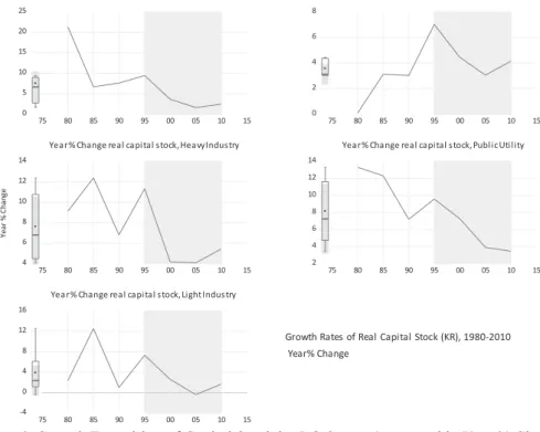
4.2 Thailand has over or under Capital Accumulation?
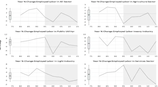
The overall labor employment has been rising to its peak of 3 percent growth in 1990. It has declined thereafter to 0% growth in the year 2000 as a result of GFC. The employment has further recovered in 2005 and declined thereafter. The agriculture employment has turned down since 1990 owing to rural- urban migration in Thailand. It has absorbed reversing ‘u-turn’ from urban to the rural area again after the AFC. It has been declining again after 2010. The service sector and heavy industrial sector has been a shock absorber of the Thai economy after the crises. The light industry is suffering from competitiveness and could not absorb employment and showing a declining trend since 1990. See Figure 5.
-1 0 1 2 3 4
75 80 85 90 95 00 05 10 15
Year % Change Empl oyed Labor i n Al l Sector Year % Change Empl oyed Labor i n Al l Sector
-4 -3 -2 -1 0 1 2 3
75 80 85 90 95 00 05 10 15
Year % Change Empl oyed Labor i n Agri cul ture Sector Year % Change Empl oyed Labor i n Agri cul ture Sector
-8 -4 0 4 8 12
75 80 85 90 95 00 05 10 15
Year % Change Employed Labor in Public Utilityr Year % Change Employed Labor in Public Utilityr
-2 0 2 4 6 8 10
75 80 85 90 95 00 05 10 15
Year % Change Employed Labor ineavy Industry Year % Change Employed Labor ineavy Industry
-2 0 2 4 6 8
75 80 85 90 95 00 05 10 15
Year % Change Employed Labor in Light Industry Year % Change Employed Labor in Light Industry
1 2 3 4 5 6
75 80 85 90 95 00 05 10 15