Prediction of Broadband Noise Generated from Turbulent Boundary Layers of a Horizontal Axis Wind Turbine Based on Wind Tunnel Test of NACA0018

(1)

NACA0018 の風洞試験に基づく水平軸風車の乱流境界層から発生する広帯域騒音の予測

佐々木壮一^＊・Zaw Moe Htet^＊＊

Prediction of Broadband Noise Generated from Turbulent Boundary Layers of a Horizontal Axis Wind Turbine Based on Wind Tunnel Test of NACA0018

by

Soichi SASAKI^*and Zaw Moe Htet^**

We expanded the blade element momentum theory (BEM) for the prediction of the broadband noise of a horizontal axis wind turbine. For the prediction of the broadband noise, the acoustic radiation from the turbulent boundary layers was applied. From the results of the wind tunnel test, NACA0018 generated the humped noise in the attached flow condition, whereas the noise spectra in the separated flow condition made the broadband noise. In this prediction methodology, the noise level of the wind turbine could be predicted by the model size of the isolated blade and the main dimensions of the objective wind turbine. At this time, the relative velocity and the angle of attack became the important parameters. We pointed out that the humped noise source in the wind turbine was made from the mid-span to the blade tip on the impeller based on this methodology.

Key words: Wind Turbine, Blade, Momentum, Aerodynamic Noise, Wind Tunnel Experiment.

1. INTRODUCTION

The horizontal axis wind turbine (HAWT) is a machine that extracts kinetic energy from the wind and converts it to mechanical energy. In Myanmar, the windy area such as sea side and flat land in the middle of the country has wind speed up to 6 m/s where wind turbine can be generated well.

However, in actual operating condition of the wind turbine, the aerodynamic noise becomes one of the important technical issue. Especially, to predict the broadband noise which is generated from the airfoil is important technical issue for the development of HAWT. The detailed review on the aerodynamics of the wind turbine rotor is described by Herman Snel ⁽¹⁾; the blade element momentum theory (BEM) in the two

dimensional has been explained in the article. The BEM is the methodology for the analysis on the fluidic properties of the blade in which the annular momentum is used for the global flow region. The BEM has been used for the analysis on the aerodynamic properties of the wind turbine, especially, for analysis of the initial development stage. Recent year, a lot of researchers are using a commercial CFD code; however, in the present stage, a lot of CFD does not guarantees the high accuracy to solve the complicated turbulent boundary layers, but cannot provide sufficient accuracy for the prediction of the aerodynamic noise. Thus, in the initial design stage, to create the suitable methodology that of not only for the aerodynamic performance but its aerodynamic noise improves the wind

平成３０年１月９日受理

＊システム科学部門（Division of System Science）

＊＊マンダレー工科大学（Mandalay Technological University）

(2)

turbine with high specifications.

In this study, we expand the blade element momentum theory for the prediction of the aerodynamic noise of the HWAT. First of all, the characteristics of NACA0018 isolated blade until the deep stall condition are clarified by the wind tunnel experiment. Moreover, for the prediction of the broadband noise, the analogy of the aerodynamic noise generated by the turbulent boundary layers is applied ⁽²⁾. Finally, we discuss the characteristics on the spectral distributions of the broadband noise which is generated by the wind turbine that of 20m diameter.

2. EXPERIMENTAL SETUP

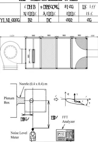
Fig.1 is the overview of the examined isolated blade. The main dimensions of the blade are listed in Table 1. We employed NACA0018 for the wind tunnel experiment. In Fig.

2, the experimental setup of the wind tunnel experiment is presented. The Reynolds number at the nozzle exit is 1.3×10⁵. The turbulence of the main flow was less than 0.5%. The leading edge of the blade is set at 450 mm downstream from the nozzle exit. A 1/2-inch microphone (Ono-Sokki, LA-4350) is set in 90° to the main flow at 1.0 m distance from the trailing edge. The frequency response is analyzed by the FFT analyzer (Ono-Sokki, CF-5210). The angle of attack is the angle between the center line of the blade and the incoming flow. The nozzle size is 400mm×400mm. The lift force and drag force which are acting on the one end of the blade can be measured by the load cell which has capacity of 25 N (Tech - Gihan, TL2B09-25N). The lift coefficient CL and drag coefficient CD

are defined as;

A V C D

A V

C_L L₂ _D 2₂ 2 ,

r

r ⁼

= (1)

where, L is the lift force, D is the drag force, ρ is the density of the fluid, V is the main flow velocity, A is the reference area.

Fig.3 is the schematic view of objective impeller of the wind turbine. The impeller is separated into 10 segments to analyze the characteristic of the fluid force and the aerodynamic performance. NACA0018 airfoil is used for every segments. The radius and the chord length of each segment are described in Table 2. Reynold number based on the chord

length at the blade tip is 4.5 × 10 ⁵.

3. BLADE ELEMENT MOMENTUM THEORY

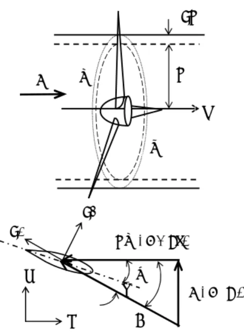
The blade element momentum theory (BEM) is used to calculate the local forces on a propeller or wind turbine blade.

The BEM can alleviate some of the difficulties in calculating the induced factors of the rotor. The velocity component of the relative velocity W is given by induced velocity factors " a "

and "a ́ " as shown in Fig. 4. The two factors are given as;

x x

y y

C a C

s f f

s s

f s

= -

= +

cos sin ' 4 sin ,

4 ² 　

(2)

t

C

Fig. 1 Overview of the examined isolated blade

Table 1 main dimensions of the blade Chord

C (mm)

Thickness T (mm)

Span L (mm)

t/C*100 (%)

NACA0018 30 5.4 100 18

1.0 m 0.45 m

X L

α Y

D V

Fig. 2 Experimental setup of the wind tunnel experiment

(3)

Here,

r c B s p

=2

where, σ is the local solidity at the position r, c is the chord length, B is the number of blades. The fluid force is assumed by Betz’s theory and Cx and Cy can be calculated by;

f f

sin cos

cos sin

D L

y

D L

x

C C

C

C C

C

+

=

-

=

(3)

Here,

' 1 1 ) ( tan 1

a a r +

= 　-

f l ,

V r rw l( )=

The angle of attack α can be calculated by the yaw angle φ and the pitch angle θ as;

q f

a = - ₍₄₎

Then, the relative velocity is expressed as Eq. (5).

(

r (1 a')

) (

² V(1 a)

)

²

W = W + + - (5)

When we take into account of the output of the wind turbine, the coefficient can be estimated by the integral from hub side to tip side as;

2 3

2

1C V R

P= _p r p (6)

Here,

ò

^×

= 1 2 dr

2 C r

C_p R _p p

p

)2

( ) 1 ( '

4a a r

C_p = - l

According to Ref. (2), the sound power radiation by a number of flat plate or airfoils, each having a surface pressure distribution caused by turbulent boundary layers, may be written as;

)

8 ₀ (

3 w

r w p

w a ^pp

W b N d

dE = φ (7)

where, E is the sound power, N is the number of blades, b is the blade span, W is the relative velocity, φpp is the wall pressure spectrum density. The wall pressure spectrum density suggested by B. D. Mugridge is given as;

3 2

10 3 W

pp = ^- r d

φ (8)

Ω

z dr

V r

ω

dD

θ dL

φ x W

α y

r Ω ( 1 +a’ )

V ( 1 –a )

Fig. 4 Schematic view of the blade element method

1000 1000 1000 1000 1000 1000 1000 1000 1000

1000

10000 500

Fig. 3 Schematic virew of the objective impeller

Table 2 Specifications of each segment

radius chord Blade shape

10.5 0.31

NACA0018

9.5 0.38

8.5 0.44

7.5 0.50

6.5 0.56

5.5 0.63

4.5 0.69

3.5 0.75

2.5 0.81

1.5 0.88

(4)

where, δ is the boundary layer displacement thickness. The boundary layer displacement thickness is evaluated by the exponential law of Eq. (9).

2

093 0

0. c R_e ^.

δ = ^- (9)

When the frequency is normalized by the chord length c and the relative velocity W, the equation (10) is established.

m o m m o

W W c c

0

w =

w (10)

We assumed that the half of sound power in the free area becomes the sound pressure level at the measurement point.

2 0

4 2

2 p

a r E

r

= p

(11)

The ratio on the sound pressure p² of the measured value of the model in the wind tunnel test to the target value of the blade element in the actual wind turbine is given by;

m pp

o pp o

m m o m o m o m o m o

r r W

W c c b b N N p p

) (

)

2 (

2 2

2

w w φ φ

÷÷ø çç ö è

÷÷ æ ø çç ö è

= æ

(12) where, subscript m is the model value, o is the objective value of the blade element for the target wind turbine. In the case of the noise level, since decibel notation is common, let me express equation (13) as logarithm.

÷÷ ø ö çç

è + æ

÷÷ø çç ö è + æ

=

m pp

o pp o

m m

o

m o m

o m

o pm

po

r r W

W

c c b

b N

L N L

) (

) log (

10 log

20 log

20

log 10 log

10 log

10

w w φ φ

(13) In the experimental analysis of the broadband noise using the scaling law, the target noise level of the wind turbine can be predicted by the model size of the isolated blade and the scale of the actual wind turbine.

4. RESULTS AND DISCUSSION

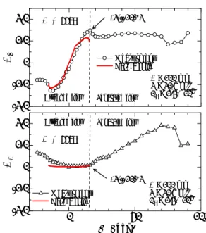
In Fig. 5, the lift coefficient and drag coefficient of NACA0018 are shown. The main flow velocity is 20.4 m/s.

The Reynolds number based on chord length is 1.3 ×10⁵. The solid line is the lift coefficient calculated by Xfoil ⁽³⁾. The circle

symbol is measured values of the lift coefficient by wind tunnel experiment. The lift coefficient of the measured value is almost same as the calculated value within the attached flow domain.

The stall point of the blade is approximately 16 °. Although measured drag coefficient is small at the attached flow domain, the measured drag coefficient agrees well with the calculated value within the attached flow domain. When the angle of attack exceeds the stall point, the drag coefficient starts to increase.

The relationship between the angle of attack and the overall noise level of the NACA0018 is presented in Fig. 6. Overall noise level does not have a big difference within the angle of attack -24° to 50 °. From the angle of attack 50 °, the noise level rises with the angle of attack. The noise level becomes

-2.0 -1.0 0 1.0 2.0

CL

Measurment Cal. (Xfoil)

C = 100 mm V = 20.4 m/s R_e = 1.3×10⁵ Stall point

Stall point Attached flow Separated flow Attached flow Separated flow

0 50 100

-2.0 -1.0 0 1.0 2.0

α , deg.

CD

Measurment Cal. (Xfoil)

C = 100 mm V = 20.4 m/s R_e = 1.3×10⁵ NACA0018

NACA0018

Fig. 5 Aerodynamic characteristics of the NACA0018

0 50 100

70 80

α , deg.

Lp, dB

C = 100 mm V = 20.4 m/s R_e = 1.3×10⁵ Attached flow Separated flow

NACA0018

BGN

Fig. 6 Noise characteristics of NACA0018

(5)

maxima at the angle of attack 70 °.

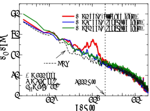
The spectral distributions of aerodynamic noise generated from NACA0018 with different angle of attack are compared in Fig. 7. The broken line is the background noise level of the wind tunnel. We can notice that the noise level in the high frequency domain than that of the 2000Hz cannot be measured because the noise level is not different from the background noise. In the angle of attack 0°, the humped noise spectra become large in where the frequency is around 1000 Hz. This noise may generate by the wake vortices in the wake of the blade. In overall noise level, the maximum noise level was at the angle of attack 70 °. The noise spectra in such a deep stall condition becomes large in the low frequency than that of the other frequency domain. This results indicated that the low

frequency noise becomes dominant for the overall noise level in the deep stall condition.

In Fig. 8, the output power of the wind turbine analyzed by the BEM is presented. The blade element in each segments is NACA0018 with pitch angle 30 °. The diameter of the impeller is 21 m; the rotation speed is 20 rpm. The common wind velocity is within 5 to 8 m/s, so that the design condition is defined as 6 m/s, whereas the wind velocity 12 m/s is defined as the off-design condition. The prediction indicates that the design condition of the pitch angle 30 ° can generate more output power than the other conditions in the off-design condition. The wind turbine can produce the maximum output power 25 kW at the wind velocity 12 m/s.

0 5 10

-20 0 20 40 60

attached flow

separated flow N = 20 rpm D = 20 m θ = 30 deg.

hub tip

V =6 m/s V =12 m/s

r , m

α, deg.

Fig. 9 Relationship between the radius from the impeller

0 5.0 10.0

0 10 20 30

N = 20 rpm D = 20 m θ = 30 deg.

hub tip

V =12 m/s V = 6m/s

r , m

W, m/s

Fig. 10 Relative velocity distributions in design and off-design operation condition

10² 10³ 10⁴

0 20 40 60 80

2000 Hz C = 100 mm

V = 20.4 m/s R_e = 1.3×10⁵

α=0 deg. (attached flow) α=24 deg. (separated flow)

α=70 deg. (separated flow)

BGN

f , Hz Lp, dB

Fig. 7 Spectral distribution of the aerodynamic noise of the NACA0018

0 10 20

0 10 20 30

V , m/s

L, kW

12 deg.

18 deg.

24 deg.

30 deg.

36 deg.

N = 20 rpm D = 21 m

Fig. 8 Output power of the wind turbine

(6)

In Fig. 9, the relationship between the radius from the impeller of the wind turbine and the angle of attack in each blade element is shown. The circle symbol is the design condition (6 m/s); the rectangular symbol is the off-design condition (12 m/s). In the design condition, most of the blade elements become the attached flow. In the off-design condition, the flow regime becomes the separated flow condition from the mid-span to the hub of the impeller. The relative velocity distributions in each operation condition are compared in Fig.

10. The relative velocity in the off-design condition becomes fast then that of the design condition. The both velocity distributions increases from hub side to the blade tip.

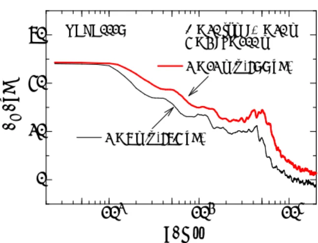
In Fig. 11, the predicted noise spectra generated from the wind turbine in the different operation condition are compared.

The thin black line is the design condition; the thick red line is the off-design condition. In the both operation conditions, the noise level becomes large in the vicinity of 4000 Hz. This humped noise may the broadband noise which is generated by the Karman Vortex shedding. The noise spectra in each span position analyzed by the BEM is shown in Fig. 12. The distance between the sound source and the microphone assumed 100 m. The predicted noise spectra indicated that the noise spectra become broadband noise at the hub side whereas the blade elements from the tip side to mid span generate the hump noise at high frequency domain.

5. SUMMARY

We proposed the prediction methodology for the broadband noise generated by the wind turbine based on the blade element momentum theory. From the results of the wind tunnel test, NACA0018 generated the humped noise in the attached flow condition, whereas the blade generated the broadband noise in the separated flow condition. Moreover, in the deep stall condition, the broadband noise in the low frequency domain increased. The broadband noise in the off-design condition became large than that of the design condition. We clarified that the humped noise source in the wind turbine was made from the mid-span to the blade tip on the impeller.

REFARENCE

(1) H. Snel, “Review of the Present Status of Rotor Aerodynamics,” Wind Energy, 1, pp. 46-69, 1998 (2) B. D. Mugridge. “Acoustic radiation from aerofoils with

turbulent boundary layers,” Journal Sound Vibration, (1971) 16 (4), 593-614.

(3) NACA4 digit airfoil generator,

http://www.airfoiltools.com/airfoil/naca4digit, accessed 25. October. 2017.

10² 10³ 10⁴

0 20 40 60

f , Hz Lp, dB

V = 6 m/s (56.4 dB)

N = 20 rpm ; D = 20 m Z = 3 ; r = 100 m NACA0018

V = 12 m/s (58.8 dB)

Fig. 11 Noise spectra generated from the wind turbine in the design and off-design operation condition

10² 10³ 10⁴

-20 0 20 40 60