The fully developed laminar heat transfer to non-Newtonian fluids flowing in a concentric annulus with a moving core is analyzed by taking into account the viscous dissipation of the flowing fluid.

Fully developed laminar heat transfer to non-Newtonian fluids flowing in a concentric annulus with a moving core

(The case of first kind of thermal boundary condition)

by

Odgerel Jambal*, Toru Shigechi**, Ganbat Davaa*, Satoru Momoki** and Tomokazu Yamamoto*

The fully developed laminar heat transfer to non-Newtonian fluids flowing in a concentric annulus with a moving core is analyzed by taking into account the viscous dissipation of the flowing fluid.

Applying the shear stress described by the modified power-law model, the energy equation together with the fully developed velocity profile is solved numerically for the thermal boundary conditions of the tube walls being kept at constant but different temperatures. The effects of the flow index, the relative velocity of the moving core, the dimensionless shear rate parameter and the Brinkman number on the temperature distribution and Nusselt numbers at the tube walls are discussed.

1. Introduction

The problems of the fully developed heat trans- fer to non-Newtonian fluids in a concentric an- nulus with an axially moving core were studied previously[lj-[2j for the thermal boundary condi- tion of constant heat flux at either tube wall.

In this paper, the fully developed heat transfer . is studied for the thermal boundary condition of the tube walls being kept at constant but differ- ent temperatures or for the first kind of boundary condition [3] . The case of the inner tube wall tem- perature being kept higher than that of the outer tube wall is referred to CASE A and the counter part is referred to CASE B. Because of the space restraint only CASE A has been discussed in the present paper.

Applying the velocity profile of the modi- fied power law fluids obtained in the previous report[4j, the energy equation including the viscous dissipation term is solved numerically.

The effects of the relative velocity of the moving core, the flow index and the dimensionless shear rate parameter and the Brinkman number on the temperature distribution and Nusselt number are discussed.

Nomenclature

Br Brinkman number

specific heat at constant pressure hydraulic diameter = 2(R

_{o -}

R

_{i )}

k thermal conductivity n flow index

Nu Nusselt number r radial coordinate

r* dimensionless radial coordinate R tube radius

T temperature

u fully developed velocity profile

Urn

average velocity of the fluid u* dimensionless velocity (=u/u

rn )

Greek Symbols a radius ratio

(3 dimensionless shear rate parameter 'rJa apparent viscosity

'rJ~

dimensionless apparent viscosity 'rJo : viscosity at zero shear rate p density

T

shear stress

() dimensionless temperature

~

transformed dimensionless radial coordinate = [2(1 - a)r* - exJl(1 - ex) Subscripts

b bulk

i inner wall or inner tube o outer wall or outer tube 2. Analysis

The geometrical configuration and the coordi- nate system for the analysis are shown in Fig.l.

Received on Oct. 24, 2003

*

Graduate student, Graduate School of Science and Technology

**

Department of Mechanical Systems Engineering

Fixed tube

Modified power law r fluid flow

•

Moving Core

f---_~u

Fig.1 Geometrical configuration The assumptions and conditions used in the

analysis are:

• The flow is steady, laminar and fully devel- oped hydrodynamically.

The bulk temperature is defined as

(7)

• The fluid is non-Newtonian with constant physical properties. The shear stress may be described by the modified power-law model.

• The body forces and the fluid axial heat con- duction are neglected.

The N usselt numbers at the walls are Nu . = hjDh

J -

k

where j = i for the inner tube wall and j =

0

for the outer tube wall and

The energy equation together with the assump- tions above is written as

{ T = T

ⁱ

at r = R

ⁱ

(2) T = To at r = R o

The velocity, u, of the modified power-law flu- ids in concentric annuli with moving cores was evaluated and reported in the previous paper(l).

The following dimensionless quantities are in- troduced

k~~ (raT) +T ^{du =} 0

rar ar dr

The thermal boundary conditions are:

CASE A

(1)

(8)

(9) (10) (11) where

T

in Eq.(I) is the shear stress defined by du

T

== ''la dr ⁽³⁾

where ''la is the apparent viscosity defined as

Dimensionless apparent viscosity,

'TJ~,

is defined as

for n > 1, (13) for n < 1, (12)

for n < 1, (14)

* 'TJo

'TJ = 1+13

'TJ* = 'TJo (1 +~)

for n < 1, (4)

_ 'TJo

'TJa = ₁ +

^'!JQ_m ^Idu._dr^{11- n}

( m IdUln-1)

'TJa == 'TJo 1 + ^'TJo dr ^{for n > 1. (5)}

I

^du*

I

ⁿ-¹

* _ 'TJa 13 + dT*

'TJa = 'TJ* = 13 + ^{1 for n> 1 (15)}

The substitution of the above quantities into the dimensional formulation gives

~ ~ ^{(r* of) ) +} Br7]* (dU*)

²

= 0 (16)

r* or* or* dr*

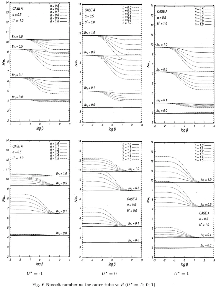
In these figures the Nusselt numbers are shown as a function of the dimensionless shear rate, {3, and the Brinkman number is a parameter. With an increase in Br, the Nusselt number at the inner tube decreases while N

Uo

increases.

are

Nusselt number at the inner and outer tube walls

References

4. Conclusions

The fully developed laminar heat transfer of the modified power-law fluids in a concentric annulus with an axially moving core was analyzed taking into account the viscous dissipation. In this work, the numerical solutions for the thermal bound- ary condition of constant but different tempera- tures at the tube walls or for the thermal bound- ary condition of first kind were obtained. The effects of the flow index, the relative core veloc- ity, the dimensionless shear rate parameter and of the Brinkman number on the temperature distri- bution and on the Nusselt numbers at the tube walls have been discussed.

(17)

(18)

*

⁰

r =

^2(1-0)

*

¹

r =

^2(1-0)

{

f) = 1 at f) = ⁰ at

The bulk temperature in the dimensionless form is calculated as

f) - 8(I-a) j2(1~<» ^{* f) * d *}

b=

1+ a

- < > -

u r r

2(1-<»

Nu, ~ ^-1 ~ ⁸

b

::.1

^<>_

⁽¹⁹⁾

r -2(1-<»

Nu

_o

= -~ ^Of)

^I

f)b

or*

* 1

r =2(1-<»

3. Results and Discussion

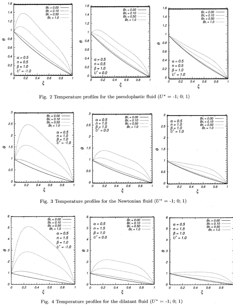
In the following figures the solutions are illus- trated for the annulus of radius ratio a = 0.5 and for the three values of the core velocity namely, U*

= -1,0 and 1. The effect of the viscous dissipation is demonstrated by the Brinkman number. The ef- fect of the Brinkman number on the temperature distributions across the channel is demonstrated in Figs.2-4. Figure 2 is for the pseudoplastic fluid of n = 0.5 and {3 = 1 while Figs. 3-4 demonstrate the temperature distributions for the Newtonian fluid n = 1 and for the dilatant fluid of n = 1.5 and {3 = 1.

.~

= 0 corresponds to the inner tube wall and

~

= 1 is the outer tube wall. The parameter in these figures are the Brinkman number. It is seen that the results for the Newtonian (n = 1) flutd and for the non-Newtonian fluids are similar qual- itatively. The dimensionless temperature increase due to the viscous dissipation is more pronounced for U* = - 1 and U* = 0 and this is attributed to the velocity gradient reported in the previous report[4j. For U* = - 1.0, f) greatly increases with an increase in Br near the moving core while for U* = 1.0, the increas in f) is small near the mov- ing core or

~

= O. Also it is seen, the temperature of the Newtonian fluid is more sensitive to the Brinkman number than that of the pseudoplastic fluids, but less than for the dilatant fluid.

Nusselt numbers at the inner core, N

Ui,

and at the outer tube wall, Nu

_{o ,}

are shown in Figs.5-6.

[1] Ganbat Davaa, Toru Shigechi and Satoru Momoki, "Heat transfer for modified power law fluids in concentric annuli with heated moving core" Reports of the Faculty of Engineering, Nagasaki University, vol. 32, No.58, p.91-98 (2002)

[2] Ganbat Davaa, Toru Shigechi and Satoru Momoki, "Heat transfer for modified power law fluids in a concentric annulus with a heated fixed outer tube" Reports of the Fac- ulty of Engineering, Nagasaki University, vol. 59, No 59, p. 33-40 (2002)

[3] R.K. Shah and A.L. London, Laminar Flow Forced Convection in Ducts, Advances in Heat Transfer, Supplement 1, Academic Press, New York (1978)

[4] Ganbat Davaa, Toru Shigechi and Satoru

Momoki, "Fluid flow for modified power

law fluids in concentric annuli with axially

moving cores", Reports of the Faculty of

Engineering, Nagasaki University, vol. 32,

No. 58, p. 83-90 (2002)

0.8 0.6

Bri = 0.00 - - : Bri = 0.10 --- ..:

Bri=0.50 Bli=1.0···

0.4 0.2

a=0.5 n=0.5 f3 = 1.0 U'

=

1.0

o

" " 1 , , , , 1

o

1.2 1.4

1.6

r---..,...

0.2 0.6 0.4

CD 0.8

0.8 Bri=O.OO - - Bli

=

O.10 ---.

Bli =0.50·

Bli=1.0···

0.4 0.6

;

0.2 1.2

1.6~ ~

1.4 Bri=O.OO - -

Bli=0.10 --- Bli =0.50

BIi=1.0 . 1.4

1.6

~---_--_--"ii

CD 0.8

c::b 0.8

0.6 0.6

0.4

a=0.5

0.4

n= 0.5

0.2

f3 =

1.0 ^0.2

U' = -1.0

0 " •• 1^{0" ,} 1

0 0.2 0.4 0.6 0.8

;

Fig. 2 Temperature profiles for the pseudoplastic fluid (U* = -1; 0; 1)

0.8

0.4 0.6

~

0.2 0.5

0.4 0.6 0.8 0.2

;

0.5

0.4 0.6 0.8

;

0.2 0.5

3 3

BIi=O.OO - - BIi=O.OO - - 3

Bli

=

O. 10 ---.

a=0.5

Bri

=

0.10 ---.

a=0.5

Bri=O.OO - -

2.5 ^Bri

=

0.50

n= 1.0

Bli =0.50 ... Bli

=

0.10 ---.

Bli

=

1.0 2.5

f3 = 1.0

Bri

=

1.0 2.5

n= 1.0

Bri

=

0.50

u' = 0.0 f3.= 1.0

^Bri

=

1.0 .. ····

a=0.5 U = 1.0

2

n = 1.0

2

f3 = 1.0

²

U· = -1.0

CD 1.5 _CD 1.5 _CD 1.5

Fig. 3 Temperature profiles for the Newtonian fluid (U* = -1; 0; 1)

BIi=O.OO - - Bli

=

0.10 ---. -

Bli

=

0.50 -

Bri

=

1.0"

0.8

6 6

BIi=O.OO - - BIi=O.OO - ' -

Bli

=

0.10 ^---

a=0.5

^Bli

=

0.10 ---

a=0.5

Bli =0.50 Bli=0.50

Bli

=

1.0 5

n= 1.5

Bli

=

1.0 .. 5

n= 1.5

a=0.5 /3= ^1.0 /3 = 1.0

= 1.5

₄

^U'=O.O U' = 1.0

= 1.0

⁴

= -1.0

<:1:>3 CD3

2 2

0.4 0.6 0.2 2

Ol....o......J....L...-......L..~~..t==;;;..;J

o

4 5

6,...---T---r----r--or---...,

CD3

Fig. 4 Temperature profiles for the dilatant fluid (U* = -1; 0; 1)

·50 -50

CASE A n 0.5 ---- CASE A n 0.5 ----

-60

a=0.5 n 0.6 -.--

_-60

a= 0.5 n 0.6

-c--

n 0.7 ... n 0.7

U· =-1.0 n 0.8··· _U' =0.0 n 0.8···

n 0.9 ---. n 0.9 ---.

n 1.0- n 1 . 0 -

·70 -70

-3 -2 -1 0 2 3 -3 ·2 -1 0 2 3

log~ log~

10 ₁₀

10,...-_-,...--~-~-"T"'""---'i

Sri=

1.0

-10

-20

~

^-30

-40

-50

CASE A n 0.5 ----

-60

a=0.5 n 0.6 ----

n 0.7 ...

U·=

1.0 n 0.8···-··

n 0.9 --- n 1 . 0 -

-70

-3 -2 -1 0 2

log~

10

Sri=

0.0

Sri

= 0.0

/ ',.,-

./,,/ _.-.-'-'-'-'-'-'-'-'-

._,,{&~~;i;::-~:~~:~:~.~·~:~:=~~:~-=~~.~~:-

10F---_-_-,...--~-"T"'""____;

Sri

=

0.0

Sn =0.5

-20 Sri

= ^1.0

-10

-40

~

^-30 Sri=

0.5

10,...---~-~-"T"'""""'O;

Sri

=

0.0 Sri=0.0

-20

-40 -10

~

^-30

3 r - . Sn -

0.5

CASE A a=0.5

U·

= 1.0

I- ~>::;.

.

-60 -50 -40

n 1.0-- n 1.1 --- n

1.2···

n 1.3 n 1.4 ---- n 1.5 ----

-70'--_.l....-_.L.-_",,--,-_""--'-, - - ' - - - '

-3 ·2 -1 0 1 2

log~

-20

. 1O:::::::"/~{ij!~'flJ,.

⁼

^1.0

....

,.

; . ; i

;

/.'

.' / .'

.'

,

,,/ "

~

^-30

2 Sri=

0.5

Sri

-0.1

a=0.5 U· =0.0

n=I.0- n= 1.1 ---.

n= 1.2 . n= 1.3

n

⁼

1.4 ---- n= 1.5 ----

,. ,.

-1 0

log~

-2 -50 -40 -10

-60 -20

.70'---_'---_.l....-_.L.-_""--'-_-'---' -3

3 2 Sri

= 0.5

Sri

= 1.0

a=0.5 U· =-1.0

n=I.0- n = 1.1 ---.

n=

1.2 .

n= 1.3 . n = 1.4 -.--- n= 1.5 ----

-1 0

log

_~

-2

-70'--_.l....-_.L.-_""--'-_""--'-_-'---' -3

-50

-60

·10

·20

U* =-1 U* = 0 U*= 1

Fig. 5 Nusseltnumber at the inner tube vs {3 (U* = ^{-1; 0; 1)}

1 4 1 " " - - _ - _ - _ - _ - , . -... 141""--_-,.--,.--,.--,.-... 1 4 1 " " - - _ - _ - _ - _ - , . -...

CASE A

13

a=0.5

12

U' = -1.0

n =0.5 -.--- n = ^{0.6 ----} n

⁼

0.7 . n=0.8 n=0.9 ---.

n=1.0-

CASE A

13

a=0.5

12 U'

=0.0

n=0.5 ----

n = 0.6 ---- n=O.7 n=0.8···

n=0.9 --- n=1.0-

CASE A

13

a=0.5

12

U' = 1.0

n = 0.5 ---.-.- n = 0.6 -.--.- n

=

0.7 . n=0.8 -···

n = 0.9 ---.

n=1.0-

3 2

Bro=

1.0

CASE A a=0.5

U'=

1.0 n=1.0- n= 1.1 ---.

n= 1.2 . n = 1.3 . n = 1.4 -.--.- n = 1.5 ----

...

-1 0

log~

·~~:~::~~~s~~.~:.~~---

"~'...""'"

":::.:::~:~ ^-- --._---_._--

-2 6

Bro

= ^0.1

Br

o

= 0.5

6 9

5

3 B,.o = 0.0

2"'--_~...,.~-~-~-~- -3

Br

o

= 0.0

3

t - - - ' - : - - - j

5 -. - - - -

---

^..,.

..._..._...._.._..,...•.~

: ....

___________________~.~.:.:.::~~~~~~;]~~~ Bro=0.1

4F---=~~

...

- - _ _ = l 12 --- •. -

10

Br

o

= 1.0

13 11

14~-r__-r__-r__-r__-r_____,

~

⁸

9 ".,"'"

~

⁸

>:~.>~,

---

----~~~·~~:~~i~~;~.,.-.. Br

o=0.5 3

Br

o

=0.1

Bro = 0.0 CASE A a=0.5 U' =0.0

2

·'~{~;~l~~~~~~.: .

\", .

6 Br.

= 0.1

5

4 Bro

= 0.0

3

- --- ----...

^....

... ^"

4

7 - - - --

5

3 -2 7 9

Br

o

= ^0.5

10

14,...-,....--,....--,....--,....--,.----,

n=1.0- n = 1.1 ---.

13

n =

1.2 .

n= 1.3 . n= 1.4 ---.-

12 :.:.:---:~:.:.-,

n= 1.5 _._._.-

11

~~;~~·~~~:·:-~;~;~--:~~--~:~;l~~~~ih,h,' ^Br

^o

^{= 1.0}

11

Br

o

= 1.0

~

⁸

~

⁸

3

Bro

= 0.0 n=1.0- n = 1.1 ---.

n= 1.2 . n= 1.3

n = ^{1.4 ----}

n=

1.5 -.--- 2

... '....

...

-$;;':;0~:~:~~::~:~~:~C~""O::7:~:~::.--~:~:7:~-

'.,...

... ^"

...-_...-... "'><>""

---~:~~~·~~:~i};;".~-Bro = 0.1

4

3 6

5 9

B,.o =0.1

6

Br

o

= ^0.5

5

B,.o = 1.0

Br

o=

0.0

3

2 ^{I I}

-3 -2 -1 0

log~

14

CASE A

13

a=0.5

12

U' =-1.0

11

10

11

~~=':"~=""=-'""~~,,~;:_c,.,.~~ Br^o

= ^1.0

10

~~~~t~~~~~~~~~:~~~~~:~~~~--~~~?~02~t~>._ ^Br

o

= ^0.5

9

~

⁸

~

⁸

3 2

-1 0

log~

-2

2' - - _ . l . . . - _ . l . . . - _ . l . . . - _ . l . . . - _ . L . . - - - I

3 -3 -1 0 2

log

~ -2

21...-_1....-_.1...-_.1...-_.1...-_.1...---1 3 -3

-1 0 2 log~

-2

21...-_1....-_1....-_1....-_1....-_.1...---1 -3

U* =-1 U* =0 U* = 1

Fig. 6 Nusselt number at the outer tube vs {3 (U* = -1; 0; 1)