数値計算
著者 Svadlenka Karel
発行年 2008‑03‑22
URL http://hdl.handle.net/2297/9574
Mathematical analysis and numerical computation of volume-constrained evolutionary problems,
involving free boundaries
(
!"$#&%' (*)+,.-)
/10232354 6*78 319:8
;=<?>?@BABC
D*E=>?@?F?G
@?H?I?J
: 0523102011
KML
: Karel ˇ Svadlenka
NPORQTS UWVXRYZQ\[ZO^]_=`Ba?b?cWd L
:
e?f gih1 Introduction 1
1.1 Introductory notes . . . . 1
1.2 Notation and function spaces . . . . 2
2 Mathematical aspects of volume preservation 5 2.1 Lagrange multiplier . . . . 5
2.2 Classification of problems . . . . 9
3 Discrete Morse flow method 11 3.1 Mathematical formulation . . . 11
3.2 Advantages and extensions of the method . . . 17
4 Problems without free boundary 19 4.1 Parabolic problem . . . 19
4.1.1 Setting . . . 19
4.1.2 Variational method . . . 20
4.1.3 The limit process . . . 23
4.1.4 H¨older continuity of weak solution . . . 28
4.1.5 Remarks on boundary conditions . . . 35
4.2 Hyperbolic problem . . . 37
4.2.1 Setting . . . 37
4.2.2 Approximate weak solution . . . 38
4.2.3 Limit process . . . 40
4.2.4 Remarks . . . 47
5 Problems with free boundary 51 5.1 Parabolic problem . . . 52
5.1.1 Model equation and its properties . . . 52
5.1.2 Existence of weak solution . . . 56
5.2 Hyperbolic problem . . . 72
5.2.1 Construction of approximate solutions . . . 72
5.2.2 Existence of solutions in one space dimension . . . 81
5.3 Appendix . . . 87
6 Numerical algorithms 97
6.1 General comments . . . 97
6.2 Finite elements with zero volume . . . 101
6.3 Appendix . . . 108
7 Numerical experiments 113 7.1 Parabolic problem without free boundary . . . 113
7.2 Hyperbolic problem without free boundary . . . 115
7.3 Parabolic problem with free boundary . . . 116
7.4 Hyperbolic problem with free boundary . . . 118
8 Conclusion 121
The object of study of the present thesis are evolutionary problems satisfying volume
preservation condition, i.e., problems whose solution have a constant value of the integral
of their graph. In particular, the following types of problems with volume constraint
are dealt with: parabolic problem (heat-type), hyperbolic problem (wave-type), parabolic
free-boundary problem (heat-type with obstacle) and hyperbolic free-boundary problem
(degenerate wave-type with obstacle). The key points are design of equations, proof of
existence of weak solutions to them and development of numerical methods and algorithms
for such problems. The main tool in both the theoretical analysis and the numerical
computation is the discrete Morse flow, a variational method consisting in discretizing
time and stating a minimization problem on each time-level. The volume constraint
appears in the equation as a nonlocal nonlinear Lagrange multiplier but it can be handled
elegantly in discrete Morse flow method by restraining the set of admissible functions for
minimization. The theory is illustrated with results of numerical experiments.
Introduction
1.1 Introductory notes
In this work, we deal with the evolution of objects of a constant volume, in particular, of surfaces that can be expressed as a graph of a scalar function. The necessity of vol- ume constraint arose in various models of physical phenomena. A typical example is an elastic membrane filled with incompressible fluid. When an outer force is applied on the membrane, it changes its shape while preserving the volume. The model equation for the membrane then has to account for this constraint.
Volume conservation in our research was first introduced in the model for a soap-film bubble moving on a flat surface. Deformations of the surface of the bubble are written in terms of a degenerate free-boundary hyperbolic equation (see [41]). However, if no condition on the volume is posed, the solution of the equation tends to zero, which means that the bubble shrinks and vanishes. In order to prevent the bubble from shrinking, the volume constraint has to be added.
The adding of the constraint is to be done at the level of deriving the model equation on the basis of physical considerations. We achieve this by imposing an appropriate limitation on the set of functions among which we look for stationary points of the Lagrangian of the system. We shall see that this results in the appearance of a new nonlocal term in the model equation. This interprets the volume constraint as an outer force acting on the whole surface.
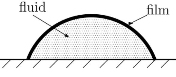
The soap bubble model became a starting point for other models, such as motion of droplets on surfaces. On the interface of the liquid forming the drop and the surrounding gas a strong layer is formed due to tension forces, and it is natural to regard the droplet as consisting of two parts: a film and liquid filling the film. In such a case, the film must preserve volume, i.e., the volume of the region between the film and the underlying surface has to be constant in time. The fluid is described by standard equations of fluid dynamics and interacts with the film via pressure forces.
We could try to model the motion of the drop by just considering the Navier-Stokes equations for the fluid. However, with this approach it is impossible to incorporate aspects like the positive contact angle of the drop or motion of dripping drops. We remark that although we have a mass-preservation condition (continuity equation) for the liquid, the film needs its own independent constraint since it determines the boundary of the domain,
1
where the fluid is moving.
We believe that such type of models combining a volume-preserving film and fluid surrounded by the film, are applicable to a wide range of phenomena. Some examples could be the flow of blood in vessels or the circulatory system as a whole, collision of objects with inner structure, propagation of waves in the sea etc. Of course, according to necessity, the coupled models may be simplified by considering the equation for the film only.
The primary aim of the present thesis is to provide mathematical analysis of such volume-preserving equations, i.e., show the existence of certain kind of solutions, their uniqueness and, if possible, regularity. However, we were able to do so for only some classes of problems by this time, leaving more complex problems for future research. One example of such unsolved problems is modelling of a droplet dripping from a ceiling, which amounts to solving a vector-valued degenerate-hyperbolic free-boundary problem.
The thesis is organized in the following way. In the beginning, we formally discuss the derivation of equations for volume-preserving phenomena from the principles of physics and hint at the relation with constrained elliptic problems. Next we introduce the main tool of this thesis, the discrete Morse flow, and show its basic properties. Chapters 4 and 5 are devoted to the analysis of basic evolutionary problems with volume constraint, considering problems without and with free boundaries, respectively. We prove existence of weak solutions and in some cases also their regularity. In the end, we make some com- ments on the numerical solution of these problems and present results of computational experiments.
1.2 Notation and function spaces
We provide a list of notations and function spaces used in the thesis.
Generally used symbols. If not stated otherwise, the symbols listed below have the following meaning:
N natural numbers (often i, j, k, l, m, n ∈ N ), R
mm-dimensional real Euclidean space ( R = R
1),
Ω bounded domain in R
mwith Lipschitz boundary, corresponding to the spatial region, where the equation is solved,
∂Ω boundary of domain Ω,
| Ω | the Lebesgue measure of Ω, Ω ¯ closure of the set Ω,
T a positive real value representing the final time, Q
Tthe open time-space cylinder (0, T ) × Ω,
V positive real value representing the volume,
K , K
Vsets of functions from certain spaces satisfying the volume constraint, u unknown function,
u
tpartial derivative of u with respect to time (=
∂u∂t),
∇ u gradient of u with respect to spatial variables (= (u
x1, u
x2, . . . , u
xm)),
∆u the Laplace operator with respect to space (=
∂∂x2u21
+ · · · +
∂x∂22u m),
u |
∂Ωthe trace of u on ∂Ω,
u
0, v
0initial data (shape and velocity, respectively),
λ Lagrange multiplier, nonlocal term originating in the volume constraint, h positive real value, time step of the discretization in time,
N natural number expressing the total number of time steps, a.e. means “almost everywhere” or “almost every”,
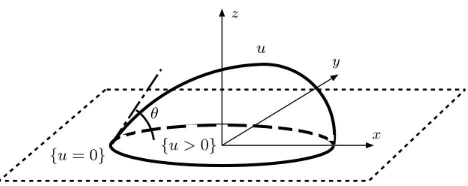
{ u > 0 } set of points (t, x) from Q
T, for which u(t, x) > 0, χ
u>0characteristic (or indicator) function of the set { u > 0 } ,
C denotes a generic positive constant, independent of parameters in question.
Function spaces. The following function spaces and their corresponding norms are used in the study (we mention only the norms used in the text). Let Ω be an open domain, k ∈ N , p ≥ 1, T > 0 and X a real Banach space with norm k · k
X.
C(Ω) continuous functions u : Ω → R ,
C
k(Ω) functions u : Ω → R that are k-times continuously differentiable, C
∞(Ω) functions u : Ω → R that are infinitely differentiable (= T
∞k=0
C
k(Ω)), C
0∞(Ω) functions from C
∞(Ω) with compact support,
L
p(Ω) functions u : Ω → R that are Lebesgue measurable and k u k
Lp(Ω)< ∞ , where k u k
Lp(Ω)= R
Ω
| u |
pdx
1/p,
L
∞(Ω) functions u : Ω → R that are Lebesgue measurable and k u k
L∞(Ω)< ∞ , where k u k
L∞(Ω)= ess sup
Ω| u | ,
W
k,p(Ω) locally summable functions u : Ω → R such that for each multiindex α with | α | ≤ k, D
αu exists in the weak sense and belongs to L
p(Ω).
The norm is defined as follows:
k u k
Wk,p(Ω)= P
|α|≤k
R
Ω
| D
αu |
pdx
1/p, k u k
Wk,∞(Ω)= P
|α|≤k
ess sup
Ω| D
αu | , H
k(Ω) = W
k,2(Ω),
H
01(Ω) the closure of C
0∞(Ω) in H
1(Ω),
L
p(0, T ; X) measurable functions u : [0, T ] → X with k u k
Lp(0,T;X)< ∞ , where k u k
Lp(0,T;X)=
R
T0
k u k
pXdt
1/p,
L
∞(0, T ; X) measurable functions u : [0, T ] → X with k u k
L∞(0,T;X)< ∞ , where k u k
L∞(0,T;X)= ess sup
0≤t≤Tk u k
X,
W
1,p(0, T ; X) functions u ∈ L
p(0, T ; X) such that u
texists in the weak sense and belongs to L
p(0, T ; X). The norm is
k u k
W1,p(0,T;X)= R
T0
k u(t) k
pX+ k u
t(t) k
pXdt
1/p,
W
1,∞(0, T ; X) functions u ∈ L
∞(0, T ; X) such that u
texists in the weak sense and belongs to L
∞(0, T ; X). The norm is
k u k
W1,∞(0,T;X)= ess sup
0≤t≤T( k u(t) k
X+ k u
t(t) k
X), H
1(0, T ; X) = W
1,2(0, T ; X),
C
0∞(Ω; R
m) functions u : Ω → R
mwith u
i∈ C
0∞(Ω), i = 1, . . . , m.
The above spaces are used also for other domains of definition, such as (0, T ) or Q
T.
We often use C
0∞(Q
T), L
2(0, T ), L
2(∂Ω), L
2(Q
T), L
∞(Q
T), H
1(Q
T), etc. The space
C
0∞([0, T ) × Ω) consists of functions from C
∞([0, T ] × Ω) that have compact support in ¯ [0, T ) × Ω, i.e., they need not vanish on { 0 } × Ω. We often use the norms of gradients in the following sense:
k∇ u k
Lp(Ω)= k |∇ u | k
Lp(Ω).
Mathematical aspects of volume preservation
In this Chapter, a typical equation of volume-preserving surface is formally derived and problems treated in the thesis are classified.
2.1 Lagrange multiplier
Ω u z
0
F
Figure 2.1: Motion of a constrained film.
We study the situation depicted in Figure 2.1 from the viewpoint of scalar functions.
A membrane is fixed on the boundary of a vessel filled with fluid. We want to know the motion of the membrane when an outer force F with potential P is applied on it. We denote by u the function expressing the shape of the membrane over a domain Ω, by ρ the area density of the membrane and by γ its elastic modulus. We assume that ρ and γ are constant, and neglect the action of the fluid on the membrane. Then the Lagrangian for the membrane can be written in the following form:
L(u) = Z
Ω
1
2 ρ(u
t)
2− 1
2 γ |∇ u |
2+ P (u)
dx. (2.1.1)
5
The equation of motion within time interval (0, T ) is given by stationary point(s) of the action
S(u) = Z
T0
L(u) dt,
that satisfy certain initial conditions, boundary condition and the volume constraint with volume V :
Z
Ω
u(t, x) dx = V ∀ t ∈ [0, T ]. (2.1.2)
This means that we look for a stationary point inside the set
K := { u; u(0, x) = u
0(x), u
t(0, x) = v
0(x), u |
∂Ω= 0, Z
Ω
u dx = V } ,
where u
0is the initial shape and v
0is the initial velocity of the membrane. For simplicity, we have prescribed homogeneous Dirichlet boundary condition.
We compute the first variation of S(u). For that purpose, it is necessary to construct perturbations that belong to K . We select a test function ϕ ∈ C
0∞((0, T ) × Ω) and use the following notation for its volume
Φ(t) = Z
Ω
ϕ(t, x) dx.
Setting
u
ε= u + εϕ 1 +
VεΦ ,
we see that this perturbation is well defined, since for small values of ε the denominator is positive, and that it belongs to K because the boundary and initial conditions are satisfied and
Z
Ω
(u + εϕ) dx = V + εΦ.
Stationary points then satisfy the identity d
dε S(u
ε) |
ε=0= 0 or equivalently lim
ε→0
S(u
ε) − S(u)
ε = 0.
We find that 0 = lim
ε→0
S(u
ε) − S(u) ε
= lim
ε→0
ρ 2ε
Z
T 0Z
Ω
h (u
t+ εϕ
t)(1 +
VεΦ) − (u + εϕ)
VεΦ
t(1 +
VεΦ)
2 2− (u
t)
2i dx dt
− lim
ε→0
γ 2ε
Z
T 0Z
Ω
h |∇ u + ε ∇ ϕ | 1 +
VεΦ
2− |∇ u |
2i dx dt + lim
ε→0
1 ε
Z
T 0Z
Ω
h
P u + εϕ 1 +
VεΦ
− P (u) i dx dt
= lim
ε→0
ρ 2ε
Z
T 0Z
Ω
(u
t+ εϕ
t+
VεΦu
t−
VεΦ
tu)
2− (u
t)
2(1 +
VεΦ)
4+ o(ε)
(1 +
VεΦ)
4dx dt
− lim
ε→0
γ 2ε
Z
T 0Z
Ω
|∇ u |
2+ 2ε ∇ u ∇ ϕ + ε
2|∇ ϕ |
2− (1 + 2
VεΦ +
Vε22Φ
2) |∇ u |
2(1 +
VεΦ)
2dx dt
+ lim
ε→0
1 ε
Z
T 0Z
Ω
P
0(u) u + εϕ 1 +
VεΦ − u
dx dt
= lim
ε→0
ρ 2ε
Z
T 0Z
Ω
2εu
tϕ
t+ 2
VεΦ(u
t)
2− 2
VεΦ
tuu
t− 4
VεΦ(u
t)
2+ o(ε)
(1 +
VεΦ)
4dx dt
− lim
ε→0
γ 2ε
Z
T 0Z
Ω
2ε ∇ u ∇ ϕ − 2
VεΦ |∇ u |
2+ o(ε) (1 +
VεΦ)
2dx dt +
Z
T 0Z
Ω
P
0(u) ϕ − 1 V Φu
dx dt
= Z
T0
Z
Ω
h ρ u
tϕ
t− 1
V u
t(Φu)
t− γ ∇ u ∇ ϕ − 1
V Φ |∇ u |
2+ P
0(u) ϕ − 1 V Φu i
dx dt
= Z
T0
Z
Ω
h ρu
tϕ
t− γ ∇ u ∇ ϕ + P
0(u)ϕ i dx dt + 1
V Z
T0
Z
Ω
h − ρu
t(uΦ)
t+ γ |∇ u |
2Φ − P
0(u)uΦ i dx dt.
Let us study the term in the last line above. If we assume that the shape of the film is smooth, we can integrate this term by parts in time, obtaining
1 V
Z
T 0Z
Ω
h − ρu
t(uΦ)
t+ γ |∇ u |
2Φ − P
0(u)uΦ i dx dt
= 1 V
Z
T 0Z
Ω
ρu
ttu + γ |∇ u |
2− F (u)u
Φ dx dt.
Thus, denoting
λ = 1 V
Z
Ω
ρu
ttu + γ |∇ u |
2− F (u)u
dx, (2.1.3)
we arrive at the relation Z
T0
Z
Ω
− ρu
tϕ
t+ γ ∇ u ∇ ϕ − F (u)ϕ − λϕ
dx dt = 0 ∀ ϕ ∈ C
0∞((0, T ) × Ω).
The strong version of the above is
ρu
tt= γ∆u + F (u) + λ(u). (2.1.4)
The analysis of this type of equations is the main object of the present thesis. We can see that we got the usual wave equation with an additional nonlocal term. This new term represents a uniform outer force on the membrane originating in the volume constraint. It may be called a Lagrange multiplier, since the same equation can be derived by a formal application of the theory of Lagrange multipliers. To see this, we consider the extremum problem for the Lagrangian once more. Since the constraint has to hold independently of time, one can judge that the Lagrange multiplier λ for the volume constraint R
Ω
u dx = V should depend on time only. Then we get the following unconstrained problem: find a stationary point of
S(u) = ˜ Z
T0
L(u) dt + Z
T0
λ(t) Z
Ω
u dx dt
among functions satisfying initial and boundary conditions. The first variation of this functional gives the same equation (2.1.4).
The usage of Lagrange multipliers is established for elliptic problems. We have, for example, the following theorem (see [8], Section 8.4).
Theorem 2.1.1. Let
K = { w ∈ H
01(Ω);
Z
Ω
G(w) dx = 0 } ,
where G : R → R is a given, smooth function with derivative g = G
0. Let u ∈ K satisfy Z
Ω
|∇ u |
2dx = min
w∈K
Z
Ω
|∇ w |
2dx.
Then there exists a real number λ such that Z
Ω
∇ u ∇ v dx = λ Z
Ω
g(u)v dx for all v ∈ H
01(Ω).
This means that u is a weak solution of the boundary-value problem
− ∆u = λg(u) in Ω,
u = 0 on ∂Ω.
In our case G(u) = u − V / | Ω | and g(u) = 1, which shows the correspondence of this equation to (2.1.4).
In proving the above theorem, one finds the Lagrange multiplier has the form λ =
R
Ω
∇ u ∇ w dx R
Ω
g(u)w dx ,
for any function w ∈ H
01(Ω), which gives a nonzero denominator. If we take w = u and consider our case, we get
λ = R
Ω
∇ u ∇ u dx R
Ω
g(u)u dx = R
Ω
|∇ u |
2dx R
Ω
u dx = 1 V
Z
Ω
|∇ u |
2dx, again corresponding to (2.1.3).
We would like to extend the theory from Theorem 2.1.1 to evolutionary equations of parabolic and hyperbolic type. Generalization of the volume constraint to general integral constraints is also a matter of interest. In order to achieve this, we approximate the evolutionary problem by a sequence of elliptic minimization problems. For the elliptic problems, we can use Theorem 2.1.1, which gives time-discrete Lagrange multipliers and time-discrete weak formulation. Taking the discretization parameter to zero, we obtain a weak solution of target equation (2.1.4). This method is called the discrete Morse flow and its basic features are explained in the next Chapter 3. Before doing so, we summarize and sort various types of problems studied in this work.
2.2 Classification of problems
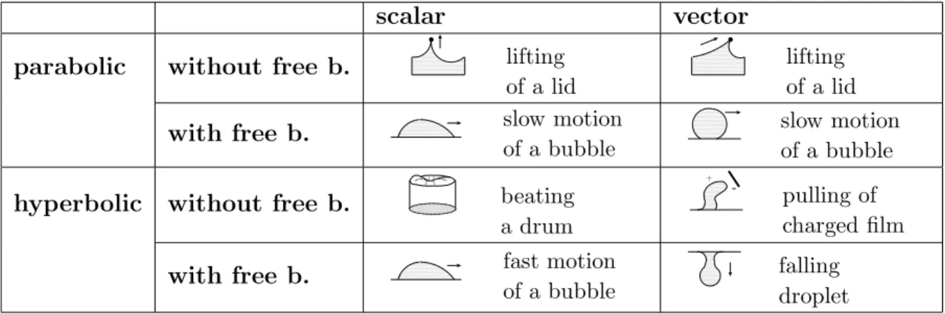
Problem (2.1.4) is of hyperbolic type but we are going to consider also other classes of problems. Although, as mentioned in the Introduction, the final aim are vector-valued problems, here we confine ourselves to problems for scalar functions. We divide them into parabolic and hyperbolic problems. Inside these groups we consider problems without and with free boundary. The parabolic problems are represented by a heat-type problem, whereas we chose a wave-type problem as an example of hyperbolic problems. A term standing for a solution-dependent outer force is added in both cases. Free-boundary problems are represented by an obstacle-type problem. The classification is featured in Table 2.1, including physical examples for each case.
scalar vector
parabolic without free b. lifting of a lid
lifting of a lid with free b. slow motion
of a bubble
slow motion of a bubble hyperbolic without free b. beating
a drum
+
pulling of charged film with free b. fast motion
of a bubble
falling droplet
Table 2.1: Classification of problems.
The example for the parabolic problem without free boundary imagines a glass filled
to the brim with water and tightly covered by an elastic membrane like a lid. This lid
is picked at some place and slowly lifted. We are then interested in the evolution of the shape of the membrane.
Parabolic free boundary problems are represented by an example of slow motion of a droplet (or a bubble), caused, for example, by chemical nonhomogeneity of the underlying surface (see Section 5.3).
Examples for hyperbolic problems can be taken the same as in the parabolic case, but with greater speed causing oscillations. We have also included two different examples for the vector-valued case: one describes the deformation and motion of a soap film caused by static electricity (sugar can be added to the soapy water in order to make it electrically active), and the other deals with a water droplet dripping from a horizontal plane.
The model for moving droplet is explained in some more detail in Section 5.3 and
additional information on some of the other examples can be found in Chapter 7.
Discrete Morse flow method
In this Chapter we explain the basic ideas and properties of the variational method called discrete Morse flow, reflecting upon its applicability to volume-constrained problems and, eventually, to free-boundary problems. This method solves time-dependent problems with differential operators concerning space variables in divergence form by discretizing time and defining a sequence of minimization problems approximating the original problem.
The corresponding minimizers are then interpolated with respect to time and discretiza- tion parameter is sent to zero.
The method was first introduced in [20] by N. Kikuchi for parabolic problems and applied to hyperbolic problems in [15], [18], [21], [27], [29], [31], [39] and other papers. It was also applied to numerical solutions of free-boundary problems, e.g., in [28], [30] and [43]. Extension to volume-preserving problems is addressed in [36], [37], [41] or [35]. We did not find any references to volume-constrained hyperbolic problems in the literature, which would be close to our approach. Representative works dealing with the problem of volume constraint in evolution equations include, for example, [3] and [16]. However, the approaches to the problems used there are fundamentally different than our own. A completely different approach that was successful in analyzing large classes of constrained evolutionary problems is the subdifferential technique using Yosida approximations (see [2], [5], [26], etc.). Nevertheless, this method works only on the abstract level, having no possibility to be applied in numerical computations. Moreover, it strongly relies on convex structure of solved problems. We shall discuss the features of this method more in detail in Section 5.1.
3.1 Mathematical formulation
We shall explain the details on the example of the wave equation. It is considered in a bounded domain Ω ⊂ R
mwith smooth boundary ∂ Ω, on which homogeneous Dirichlet boundary condition is given.
Initial position u
0∈ H
01(Ω) and initial velocity v
0∈ H
01(Ω) are prescribed. Therefore, we have the following problem:
11
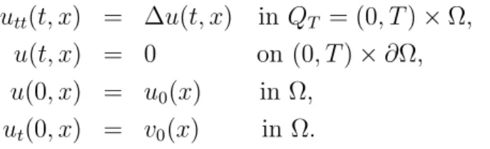
u
tt(t, x) = ∆u(t, x) in Q
T= (0, T ) × Ω, (3.1.1)
u(t, x) = 0 on (0, T ) × ∂Ω, (3.1.2)
u(0, x) = u
0(x) in Ω, (3.1.3)
u
t(0, x) = v
0(x) in Ω. (3.1.4)
First, we fix a natural number N > 0, determine the time step h = T /N and put u
1(x) = u
0(x) + hv
0(x). Function u
0corresponds to the approximate solution at time level t = 0, while function u
1is the approximate solution at time level t = h. We define the approximate solution u
non further time levels t = nh for n = 2, 3, . . . , N , to be the minimizer of the following functional in H
01(Ω):
J
n(u) = Z
Ω
| u − 2u
n−1+ u
n−2|
22h
2dx + 1
2 Z
Ω
|∇ u |
2dx. (3.1.5) We observe that the second term of the functional is lower-semicontinuous with respect to sequentially weak convergence in H
1(Ω) and the first term is continuous in L
2(Ω). The existence of minimizers then follows immediately from the fact that the functionals are bounded from below for each n = 2, 3, . . . , N . This is a crucial advantage over the contin- uous version of this functional, the Lagrangian introduced in (2.1.1). Of course, if other terms, representing outer forces etc. are present, we have to make certain assumptions concerning these terms in order to get the existence of a minimizer.
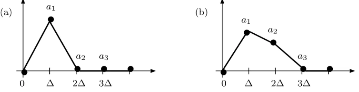
u u
t t
u
h: u ¯
h:
u1 u0
u2
u3 u4
u0 u1
u2 u3
u4
0 h 2h 3h 4h 0
h 2h 3h 4h
Figure 3.1: Interpolation of minimizers.
As the next step, we define the approximate solutions ¯ u
hand u
hthrough interpolation of the minimizers { u
n}
Nn=0in time. The interpolation is schematically demonstrated in Figure 3.1 and precisely given by
¯
u
h(t, x) =
( u
0(x), t = 0
u
n(x), t ∈ ((n − 1)h, nh], n = 1, . . . , N, (3.1.6) u
h(t, x) =
( u
0(x), t = 0
t−(n−1)h
h
u
n(x) +
nh−thu
n−1(x), t ∈ ((n − 1)h, nh], n = 1, . . . , N.
Since u
nis a minimizer of J
n, the first variation of J
nat u
nvanishes. Thus, for any
ϕ ∈ H
01(Ω) we have
0 = d
dε J
n(u
n+ εϕ) |
ε=0= lim
ε→0
J
n(u
n+ εϕ) − J
n(u
n) ε
= lim
ε→0
1 ε
Z
Ω
| u
n+ εϕ − 2u
n−1+ u
n−2|
2− | u
n− 2u
n−1+ u
n−2|
22h
2dx
+ lim
ε→0
1 2ε
Z
Ω
|∇ u
n+ ε ∇ ϕ |
2− |∇ u
n|
2dx
= lim
ε→0
Z
Ω
(2u
n+ εϕ − 4u
n−1+ 2u
n−2)ϕ
2h
2dx + lim
ε→0
1 2
Z
Ω
2 ∇ u
n∇ ϕ + ε |∇ ϕ |
2dx
= Z
Ω
u
n− 2u
n−1+ u
n−2h
2ϕ dx + Z
Ω
∇ u
n∇ ϕ dx. (3.1.7)
Using the definition of ¯ u
hand u
hin (3.1.6), this can be rewritten as Z
Ω
h u
ht(t) − u
ht(t − h)
h ϕ + ∇ u ¯
h(t) ∇ ϕ i
dx = 0 for a.e. t ∈ (h, T ) ∀ ϕ ∈ H
01(Ω).
We note that the above relation holds also when multiplied by any function ˜ ϕ ∈ C([0, T ]).
Hence, integrating over the time interval (h, T ) and using a standard density argument, we arrive at
Z
T hZ
Ω
h u
ht(t) − u
ht(t − h)
h ϕ + ∇ u ¯
h∇ ϕ i
dx dt = 0 ∀ ϕ ∈ L
2(0, T ; H
01(Ω)). (3.1.8) Now, we would like to take the time step to zero. To be able to do so, some estimate on the approximate solutions is needed. We state it in the following Lemma.
Lemma 3.1.1. Suppose Ω is a bounded domain with smooth boundary. Let J
n, n = 2, . . . , N , be the functionals defined by (3.1.5) and let u
nbe corresponding minimizers in H
01(Ω). Define functions u ¯
hand u
hby (3.1.6) and assume h ≤ 1. Then the following estimate holds
k u
ht(t) k
L2(Ω)+ k∇ u ¯
h(t) k
L2(Ω)≤ C
Efor a.e. t ∈ (0, T ), (3.1.9) where constant C
Edepends on H
1-norms of the initial data but is independent of h.
Proof. Estimate of such kind is usually derived by testing the equation by the time- derivative of solution. Here it amounts to setting ϕ := u
n− u
n−1in (3.1.7). This yields
Z
Ω
u
n− 2u
n−1+ u
n−2h
2(u
n− u
n−1) dx + Z
Ω
( ∇ u
n− ∇ u
n−1) ∇ u
ndx = 0.
We employ the inequality a
22 − b
22 ≤ (a − b)a, ∀ a, b ∈ R , (3.1.10)
to find that for each n = 2, 3, . . . , N , the following holds:
Z
Ω
h u
n− u
n−1h
2− u
n−1− u
n−2h
2+ |∇ u
n|
2− |∇ u
n−1|
2i
dx ≤ 0 Z
Ω
h u
n− u
n−1h
2+ |∇ u
n|
2i dx ≤
Z
Ω
h u
n−1− u
n−2h
2+ |∇ u
n−1|
2i dx.
These inequalities are summed from n = 2 to an arbitrary integer k ≤ N . Since the terms in between cancel, we obtain
Z
Ω
h u
k− u
k−1h
2+ |∇ u
k|
2i
dx ≤ Z
Ω
h u
1− u
0h
2+ |∇ u
1|
2i dx
= Z
Ω
(v
0)
2+ |∇ u
0+ h ∇ v
0|
2dx
≤ Z
Ω
(v
0)
2+ 2 |∇ u
0|
2+ 2h
2|∇ v
0|
2dx
≤ 2 k u
0k
2H1(Ω)+ 2 k v
0k
2H1(Ω). This is already the desired estimate (3.1.9), because
u
ht(t) = u
k− u
k−1h for t ∈ ((k − 1)h, kh), k = 1, 2, . . . , N.
2 Thanks to estimate (3.1.9), we can apply the theorem by Eberlein and Shmulyan (see [42], Appendix to Chapter V) to extract a subsequence {∇ u ¯
hk}
k∈Nwhich converges weakly in L
2(Q
T) to a function v. From the sequence { h
k}
k∈Nobtained in this way, we can extract another subsequence { h
kl}
l∈Nso that { u
htkl}
l∈Nconverges weakly in L
2(Q
T) to a function U . In the sequel, we often use this logic but we shall omit this lengthy explanation and subscripts and simply write
∇ u ¯
h* v in (L
2(Q
T))
m, (3.1.11)
u
ht* U in L
2(Q
T). (3.1.12)
We should now show that there is a function u ∈ L
2(0, T ; H
01(Ω)) such that v = ∇ u and U = u
tin L
2(Q
T). To this end, a more detailed analysis is needed. First, we estimate the norm of the difference of the approximate functions ¯ u
hand u
h. Let t ∈ ((n − 1)h, nh).
Then
k u ¯
h(t) − u
h(t) k
2L2(Ω)= Z
Ω
(¯ u
h− u
h)
2dx
= Z
Ω
u
n− t − (n − 1)h
h u
n− nh − t
h u
n−12dx
= Z
Ω
nh − t h
2(u
n− u
n−1)
2dx
≤ Z
Ω
(u
n− u
n−1)
2dx = h
2Z
Ω
(u
ht)
2dx
≤ C
E2h
2.
This means that
k u ¯
h(t) − u
h(t) k
L2(Ω)≤ Ch for a.e. t ∈ (0, T ).
We have further
k u
hk
2L2(QT)− k u ¯
hk
2L2(QT)= Z
T0
Z
Ω
(u
h)
2− (¯ u
h)
2dx dt
=
N
X
n=1
Z
nh (n−1)hZ
Ω
h t − (n − 1)h
h u
n− nh − t h u
n−1 2− u
2ni dx dt
=
N
X
n=1
Z
nh (n−1)hZ
Ω
h (t − (n − 1)h)
2− h
2h
2u
2n+ 2 (t − (n − 1)h)(nh − t)
h
2u
nu
n−1+ (nh − t)
2h
2u
2n−1i
dx dt
=
N
X
n=1
Z
Ω
− 2h
3 u
2n+ h
3 u
nu
n−1+ h 3 u
2n−1dx
≤ h 6
N
X
n=1
Z
Ω
− 4u
2n+ u
2n+ u
2n−1+ 2u
2n−1dx
= h
2
N
X
n=1
Z
Ω
( − u
2n+ u
2n−1) dx = h 2
Z
Ω
(u
20− u
2N) dx
≤ h
2 k u
0k
2L2(Ω). In the same way we get also
k∇ u
hk
2L2(QT)− k∇ u ¯
hk
2L2(QT)≤ h
2 k∇ u
0k
2L2(Ω).
Finally, from Poincar´e’s inequality (see [8], Section 5.6) we know that there is a universal constant C
Pso that
k u
hk
L2(QT)≤ C
Pk∇ u
hk
L2(QT)for all h ∈ (0, 1). (3.1.13) We summarize the results for future use. We remark that the results of the following Lemma rely only on the interpolation (3.1.6) and are independent of the problem under consideration, a fact frequently used later on.
Lemma 3.1.2. Let u ¯
hand u
hbe defined by (3.1.6). Then the following relations hold.
k u ¯
h(t) − u
h(t) k
L2(Ω)≤ h k u
ht(t) k
L2(Ω)for a.e. t ∈ (0, T ), (3.1.14) k u
hk
2L2(QT)≤ k u ¯
hk
2L2(QT)+ h
2 k u
0k
2L2(Ω), (3.1.15) k∇ u
hk
2L2(QT)≤ k∇ u ¯
hk
2L2(QT)+ h
2 k∇ u
0k
2L2(Ω). (3.1.16)
Now, (3.1.9), (3.1.16) and (3.1.13) imply that u
his uniformly bounded in H
1(Q
T).
Therefore, there is a weakly convergent subsequence in H
1(Q
T) and, by Rellich theorem (see [8], Section 5.7), a strongly converging subsequence in L
2(Q
T) (we always mean
“subsequence of the last obtained sequence”). Let us denote the cluster function as u:
u
h* u weakly in H
1(Q
T). (3.1.17) Because of (3.1.12), U = u
tholds almost everywhere. Moreover, from (3.1.11) for any ϕ ∈ C
0∞(Q
T)
Z
T 0Z
Ω
∂ u ¯
h∂x
i− ∂u
h∂x
iϕ dx dt → Z
T0
Z
Ω
v
i− ∂u
∂x
iϕ dx dt as h → 0+, while at the same time
Z
T 0Z
Ω
∂ u ¯
h∂x
i− ∂u
h∂x
iϕ dx dt = − Z
T0
Z
Ω
(¯ u
h− u
h) ∂ϕ
∂x
idx dt → 0 as h → 0+
by (3.1.14). This means that v = ∇ u almost everywhere in Q
T.
We have shown in this way that there is a function u ∈ H
1(Q
T), such that
∇ u ¯
h* ∇ u in (L
2(Q
T))
m, (3.1.18)
u
ht* u
tin L
2(Q
T). (3.1.19)
Now, we can pass to limit in (3.1.8) as h → 0+. We shall, for the time being, consider a test function ϕ belonging to C
0∞([0, T ) × Ω). To begin with, we have
Z
T hZ
Ω
∇ u ¯
h∇ ϕ dx dt = Z
T0
Z
Ω
∇ u ¯
h∇ ϕ dx dt − Z
h0
Z
Ω
∇ u ¯
h∇ ϕ dx dt
→ Z
T0
Z
Ω
∇ u ∇ ϕ dx dt as h → 0+, (3.1.20)
because of the boundedness (3.1.9) of ∇ u ¯
h:
Z
h0
Z
Ω
∇ u ¯
h∇ ϕ dx dt ≤
Z
h 0Z
Ω
|∇ u ¯
h|
2dx
1/2Z
Ω
|∇ ϕ |
2dx
1/2dt
≤ Z
h0
p C
EC dt = Ch → 0 as h → 0 + . Moreover, we have
Z
T hZ
Ω
u
ht(t) − u
ht(t − h)
h ϕ dx dt
= Z
Th
Z
Ω
u
ht(t)
h ϕ(t) dx dt − Z
T−h0
Z
Ω
u
ht(t)
h ϕ(t + h) dx dt
= Z
T0
Z
Ω
u
ht(t) ϕ(t) − ϕ(t + h)
h dx dt −
Z
h 0Z
Ω
u
ht(t)
h ϕ(t) dx dt +
Z
T T−hZ
Ω
u
ht(t)
h ϕ(t + h) dx dt (3.1.21)
→ − Z
T0
Z
Ω
u
tϕ
tdx dt − Z
Ω
v
0ϕ(0) dx as h → 0 + .
The convergence is deduced from the following facts: (i) in the first term of (3.1.21), u
htconverges weakly and (ϕ(t) − ϕ(t + h))/h converges strongly in L
2(Q
T); (ii) in the second term, u
ht= (u
1− u
0)/h = v
0for t ∈ (0, h) ; (iii) in the third term, ϕ(t + h) = 0 for t ∈ (T − h, T ). Thus, we can finally state that
Z
T 0Z
Ω
( − u
tϕ
t+ ∇ u ∇ ϕ) dx dt − Z
Ω
v
0ϕ(0, x) dx = 0 ∀ ϕ ∈ C
0∞([0, T ) × Ω). (3.1.22) Noting that the space of functions from H
1(Q
T) with zero trace on ( { 0 } × Ω) ∪ ([0, T ] × ∂Ω) is a closed linear subspace of H
1(Q
T) and, therefore, weakly closed by Mazur’s theorem (see [8], Appendix D), we conclude by (3.1.17) that u belongs to this space. Consequently, u satisfies boundary condition (3.1.2) and initial condition (3.1.3) in the sense of traces. We remark that the convergence of traces follows also from the compactness of the trace operator T : H
1(Ω) → L
2(∂Ω). Moreover, from [8] (Section 5.9), it follows that u, as a function from H
1(0, T ; L
2(Ω)), belongs to C([0, T ]; L
2(Ω)). Thus, the initial condition (3.1.3) is satisfied even in the strong sense.
To summarize, we have proved by the discrete Morse flow method that there exists a weak solution u ∈ H
1(Q
T) to problem (3.1.1) – (3.1.4) in the sense of (3.1.22), satisfying boundary and initial conditions (3.1.2), (3.1.3) in the sense of traces.
3.2 Advantages and extensions of the method
There are certainly many different and easier ways how to achieve this result. Neverthe- less, the method of discrete Morse flow can be naturally applied to problems with volume constraint and extends even to free-boundary problems, as we shall gradually show in the following pages.
The advantage of this approach regarding volume-constrained problems, and the rea- son we have adopted it, lies in the fact that a semi-discretization of time allows us to use results from elliptic theory. Moreover, the variational principle enables us to deal with the volume constraint by incorporating the condition in the set of admissible functions.
We considered using standard methods to solve this problem, but the nonlinear and nonlocal character of the multiplier term (see (2.1.3)) complicates the situation greatly.
For example, the Galerkin approximation method yields a system of nonlinear ordinary differential equations and the existence of its solution on the whole time interval is not clear. Likewise, applying fixed point methods requires stronger assumptions on the data and fails to guarantee that the volume is preserved for approximate solutions, which makes it difficult to obtain necessary estimates. As such, these approaches do not easily yield the existence of a (weak) solution to our problem. What is more, unlike the Morse flow method, they are not suitable for numerical computations. The relation to subdifferential methods was mentioned in the beginning of this chapter.
As already intimated, we add the volume constraint into the set of admissible functions
for minimization of the time-discrete functional when solving problems with preservation
of volume. In other words, we minimize the same functional (3.1.5) in the set K = { u ∈ H
01(Ω);
Z
Ω
u dx = V } ,
instead of minimizing in H
01(Ω). The details of the analysis and results are presented in the following Chapter 4 for both parabolic and hyperbolic problems.
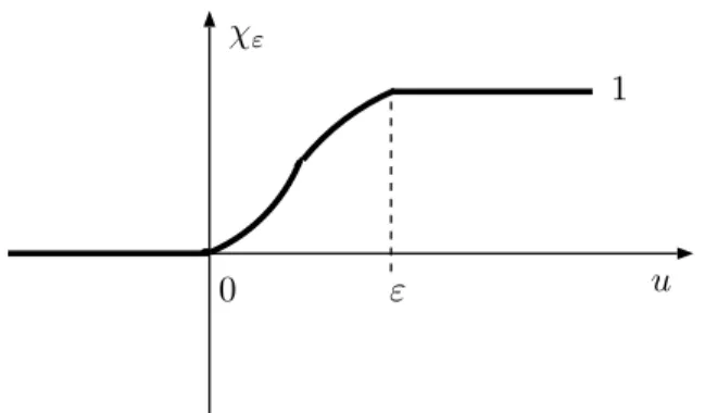
The situation becomes somewhat complicated for free-boundary problems. Let us consider an obstacle problem with a plane obstacle corresponding to the level u = 0 (think of a soap bubble on the surface of water). Assuming that there is no reflection when the soap film touches the plane (i.e., energy is lost), we show that the degenerate hyperbolic equation
χ
u>0u
tt= ∆u + γχ
0ε(u) + λ(u)χ
u>0, with λ(u) = 1 V
Z
Ω
u
ttu + |∇ u |
2+ γuχ
0ε(u) dx, is a reasonable description of the motion of the bubble. Here χ
u>0is the characteristic function of the set { (t, x); u(t, x) > 0 } (the region where the bubble sits), χ
εis its ap- propriate smoothing and γ depends on the various gas/liquid/solid surface tensions. The discrete Morse flow can be applied to this problem, too, and amounts to minimizing of
J
n(u) = Z
Ω
| u − 2u
n−1+ u
n−2|
22h
2χ
u>0dx + 1 2
Z
Ω
|∇ u |
2dx + Z
Ω
γχ
ε(u) dx in K = { u ∈ H
01(Ω);
Z
Ω
uχ
u>0dx = V } .
The obstacle condition is achieved through the characteristic functions appearing in the
admissible function set and at the discretized term of the functional. Parabolic and
hyperbolic free-boundary problems of this type are studied in Chapter 5.
Problems without free boundary
In this Chapter, we deal with the simplest version of volume-constrained problems - parabolic problems of heat type with an ‘heat source’ term and hyperbolic problems corresponding to wave equation.
4.1 Parabolic problem
4.1.1 Setting
In this part, which paraphrases paper [36], we consider the problem of finding a scalar function u : [0, T ) × Ω → R subject to the following constraints:
u
t(t, x) − ∆u(t, x) = f (t, x, u) + λ(t) (t, x) ∈ Q
T,
u(t, x) = g(x) t ∈ (0, T ), x ∈ ∂Ω, (4.1.1) u(0, x) = u
0(x) x ∈ Ω.
Throughout this section, Ω is a bounded domain in R
mwith piecewise smooth boundary
∂Ω, Q
T= (0, T ) × Ω, T > 0, and λ(t) is the Lagrange multiplier determined by the volume-preserving condition:
Z
Ω
u(t, x) dx = V (4.1.2)
for all t in the interval (0, T ) and a given volume V . The multiplier is independent of x and has the form
λ(t) = 1 V
Z
Ω