Theoretical and numerical studies of the shallow water equations with a transmission boundary condition

Theoretical and numerical studies of the shallow water equations with a transmission boundary condition

著者 エムディ マスム ムシェド

著者別表示 Md Murshed Masum journal or

publication title

博士論文要旨Abstract 学位授与番号 13301甲第5003号

学位名 博士（理学）

学位授与年月日 2019‑09‑26

URL http://hdl.handle.net/2297/00056469

Creative Commons : 表示 ‑ 非営利 ‑ 改変禁止

Dissertation Abstract

Theoretical and numerical studies of the shallow water equations with a transmission boundary

condition

Graduate School of

Natural Science & Technology Kanazawa University

Division of Mathematical and Physical Sciences

Student ID No. : 1624012011

Name : Murshed Md Masum

Chief Advisor : Professor Masato Kimura

Date of Submission (Revised version) : September 12, 2019

Abstract

In this work, the stability of the shallow water equations (SWEs) with a transmission boundary condition is studied theoretically and numerically using a suitable energy. In the theoretical part, using a suitable energy, we begin with deriving an equality which implies an energy estimate of the SWEs with the Dirichlet and the slip boundary conditions. For the SWEs with a transmission boundary condition, an inequality for the energy estimate is proved under some assumptions to be satisfied in practical computation. In the numerical part, based on the theoretical results, the energy estimate of the SWEs with a transmission boundary condition is confirmed numerically by a finite difference method (FDM) and Lagrange–Galerkin method (LGM). The choice of a positive constantc0used in the transmission boundary condition is investigated additionally. Furthermore, we present numerical results by a LGM, which are similar to those by the FDM. The computation of the SWEs with the transmission boundary condition are also made for the Bay of Bengal by a LGM with the triangular mesh. To see the performance of the LGM we have investigated the experimental order of convergence for the LGM with a suitable choice of exact solutions for five different cases of boundary setting for the norms several norms. The results are satisfactory. In order to see whether the transmission boundary condition is independent of its position or not, simulations are made in the Bay of Bengal, setting the transmission boundary condition in two different places. We have computed the mass andL²-norm ofηand the results shows that the transmission boundary condition works well numerically it is almost independent of its position.

1 Introduction

The shallow water equations (SWEs) can be considered as a coupled system of a pure convection equation for the functionϕof total wave height and a simplified Navier–Stokes equation for the velocityu= (u1, u2)^T obtained by averaging function values inx3-direction, which are often used for the simulation of tsunami/storm surge in the bay.

Figure 1: The Bay of Bengal

In such simulation there are some boundaries in the open sea, see Figure 1. In a real situation, if wave propagates towards such boundaries in the open sea, then there should not be any reflection on these boundaries.

In this study, following [?], we employ a transmission boundary con- dition on the boundaries in the open sea which is capable to remove this kind of artificial reflection.

It is to be noted here that our final goal is to develop a storm surge prediction model for the Bay of Bengal. For such models researchers, usually employ a radiation type boundary condition on the boundaries in the open sea, see, e.g., [?,?,?,?], which is very similar to the transmission boundary condition used in [?].

The transmission boundary condition of the form

u(x, t) =c(x)η(x, t)

ϕ(x, t)n(x) (1)

is often used onΓT, wherec(x) is a given positive function andη(x, t) = ϕ(x, t)−ζ(x) is the elevation from the reference height for a given depth functionζ.

In this paper, in order to understand the transmission boundary con- dition mathematically, we study the stability of the SWEs in terms of a suitable energy, and confirm the stability numerically by a finite difference method (FDM) and a finite element method (FEM).

It is to be noted here that we can show a (successful) energy estimate of the SWEs, when only the Dirichlet and the slip boundary conditions are employed, cf. Corollary??-(ii), where such discussions have been done under the periodic boundary condition, e.g., [?,?]. As far as we know, however, there is no mathematical results on the energy estimate of the SWEs with the transmission boundary condition.

Although, at present, the mathematical results do not derive the stability estimate of the SWEs with the transmission boundary condition directly, we have good information and can study the stability numerically by using the theoretical results.

It is known that the FEM is more suitable than FDM for a domain of irregular shape. As the shape of the Bay of Bengal is very irregular, the simulation of the SWEs with the transmission boundary condition are also made by a Lagrange–Galerkin method (LGM) for this domain. The LGM is a FEM based on the time discretization of the material derivative,

ϕ^k+1(x)−ϕ^k(x−u^k(x)∆t)

∆t .

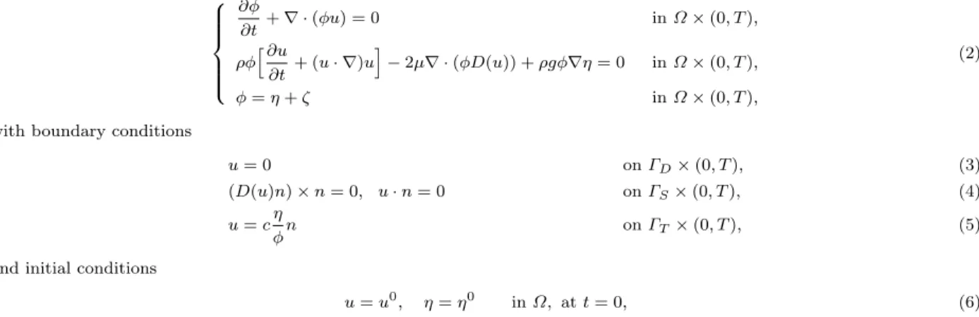
2 Statement of the problem

In this section, we state the mathematical problem to be considered in this paper. LetΩ⊂R²be a bounded domain andT a positive constant. We consider the problem : find (ϕ, u) :Ω×[0, T]→R×R² such that













∂ϕ

∂t +∇ ·(ϕu) = 0 inΩ×(0, T),

ρϕ [∂u

∂t + (u· ∇)u

]−2µ∇ ·(ϕD(u)) +ρgϕ∇η= 0 inΩ×(0, T),

ϕ=η+ζ inΩ×(0, T),

(2)

with boundary conditions

u= 0 onΓD×(0, T), (3)

(D(u)n)×n= 0, u·n= 0 onΓS×(0, T), (4)

u=cη

ϕn onΓT×(0, T), (5)

and initial conditions

u=u⁰, η=η⁰ inΩ, att= 0, (6)

whereϕis the total height of wave,u= (u1, u2)^T is the velocity,η:Ω×[0, T]→Ris the water level from the reference height, ζ(x)>0 (x∈Ω) is the depth of water from the reference height, see Figure 2,D(u) :=(

∇u+ (∇u)^T)

/2 is the strain-rate tensor,nis the unit outward normal vector to the boundary ofΩ,Γ:=∂Ω is the boundary ofΩ, we assume thatΓconsists of non-overlapped three parts,ΓD,ΓSandΓT, i.e.,Γ=ΓD∪ΓS∪ΓT,ΓD∩ΓS=∅,ΓS∩ΓT=∅,

Figure 2: Model domain

ΓT ∩ΓD =∅, the subscripts “D”, “S”, and “T” mean Dirichlet, slip, and transmission boundaries, respectively,ρ >0 is a constant which represents the density of water,µ >0 is a constant which represents the viscosity,g >0 is the acceleration due to gravity, andc(x) :=c0

√gζ(x) with a positive constantc0. In the rest of paper, we assumeζ∈C¹(Ω). It is important to note here that the equations in (??) are derived in [?] by considering one-layer viscous SWEs. It is of interest to note here that [?]

studied about the existence, uniqueness and [?] studied about the con- vergence of a finite element scheme for linearized SWEs but there is no theoretical results, as far we know, for the existence, uniqueness or regu- larity for the model (??)–(??) yet. Also it is pertinent to point out here thatϕ(x, t)>0 for allx∈Ωandt∈[0, T] can not be shown theoretically for (??)–(??), but for this problem withΓT =∅, we have the following Remark.

Remark 2.1. (Remark 3.1.1. in thesis) If Γ ∈C²,u·n≥0 onΓ,ϕ(x,0)>0 for allx∈Ω, then by the characterstic method it can be shown thatϕ(x, t)>0 for allx∈Ωandt∈[0, T].

3 Energy estimate

In this section, we define the total energy and study the stability of solu-

tions to the problem stated in Section??in terms of the energy. For a solution of (??) the total energyE(t) at timet∈[0, T]

is defined by

E(t) :=E1(t) +E2(t), (7)

whereE1(t) andE2(t) are the kinetic and the potential energies defined by E1(t) :=

∫

Ω

ρ

2ϕ|u|²dx, E2(t) :=

∫

Ω

ρg|η|² 2 dx.

Let symbolsIi(t;Γ),i= 1, . . . ,3, andI4(t;Ω),t∈[0, T], be integrals defined by I1(t;Γ) :=−ρ

2

∫

Γ

ϕ|u|²u·n ds, I2(t;Γ) :=−ρg

∫

Γ

ϕηu·n ds, I3(t;Γ) := 2µ

∫

Γ

ϕ[ D(u)n]

·u ds, I4(t;Ω) :=−2µ

∫

Ω

ϕ|D(u)|²dx.

These are used in the rest of this paper. Let us assume

ϕ∈C¹(Ω×[0, T] :R), u∈C¹(Ω×[0, T] :R²), (8) and

∂i∂ju∈C¹(Ω×[0, T] :R²) fori, j= 1,2. (9)

Theorem 3.1. (Theorem 3.2.1. in thesis)Suppose that a pair of functions(ϕ, u) :Ω×[0, T]→R×R² satisfies(??) with (??)and(??). Then, we have

d dtE(t) =

∑3 i=1

Ii(t;Γ) +I4(t;Ω). (10)

We prove Theorem??using the following lemma.

Lemma 3.2. (Lemma 3.2.2. in thesis)For the functionsϕ:Ω×[0, T]→Randu:Ω×[0, T]→R² satisfying(??), we have the following.

(i) ∂

∂t(ϕu) +∇ ·[(ϕu)⊗u] = (∂ϕ

∂t +∇ ·(ϕu) )

u+ϕ (∂u

∂t + (u· ∇)u )

, (ii)

∫

Ω

(∇ ·[(ϕu)⊗u])·udx=1 2

∫

Γ

ϕ|u|²u·nds+1 2

∫

Ω

[∇ ·(ϕu)]|u|²dx.

Proof of Theorem??. Differentiating (??) with respect tot, we get d

dtE(t) = d

dtE1(t) + d

dtE2(t). (11)

We compute _dt^dE1(t) and _dt^dE2(t) separately.

Firstly, _dt^dE1(t) is computed as follows. From Lemma??-(i) and the first equation of (??), we have

ϕ[∂u

∂t + (u· ∇)u]

= ∂

∂t(ϕu) +∇ ·[(ϕu)⊗u], which implies

ρ [∂

∂t(ϕu) +∇ ·[(ϕu)⊗u]

]−2µ∇ ·[ ϕD(u)]

+ρgϕ∇η= 0. (12)

Multiplying (??) byuand integrating with respect toxoverΩ, we get ρ

∫

Ω

[∂

∂t(ϕu)]

·u dx+ρ

∫

Ω

[∇ ·[(ϕu)⊗u]]

·u dx−2µ

∫

Ω

[∇ ·(ϕD(u))]

·u dx +ρg

∫

Ω

ϕ∇η·u dx= 0. (13)

From the equation (??) above and the next two identities:

ρ

∫

Ω

[∂

∂t(ϕu)]

·u dx+ρ

∫

Ω

[∇ ·[(ϕu)⊗u]]

·u dx

=ρ

∫

Ω

(∂ϕ

∂t|u|²+ϕ∂u

∂t ·u) dx+ρ

2

∫

Γ

ϕ|u|²u·n ds+ρ 2

∫

Ω

[∇ ·(ϕu)]

|u|²dx (from Lemma??-(ii))

=ρ

∫

Ω

(1 2

∂ϕ

∂t|u|²+ϕu·∂u

∂t )

dx+ρ 2

∫

Γ

ϕ|u|²u·n ds (from the first eq. of (??))

= d dt

[ρ 2

∫

Ω

ϕ|u|² dx ]

+ρ 2

∫

Γ

ϕ|u|²u·n ds= d

dtE1(t)−I1(t;Γ),

−2µ∫

Ω

[∇ ·(ϕD(u))

]·u dx=−2µ∫

Γ

ϕ[ D(u)n]

·u ds+ 2µ

∫

Ω

ϕ|D(u)|²dx

=−I3(t;Γ)−I4(t;Ω), we obtain

d

dtE1(t) =I1(t;Γ) +I3(t;Γ) +I4(t;Ω)−ρg

∫

Ω∇η·(ϕu)dx. (14)

Secondly, _dt^dE2(t) is computed as follows:

d

dtE2(t) = d dt

[ρg 2

∫

Ω|η|²dx ]

=ρg

∫

Ω

η∂η

∂tdx

=ρg

∫

Ω

η∂ϕ

∂tdx (from the third eq. of (??))

=ρg

∫

Ω

η[

−∇ ·(ϕu)]

dx (from the first eq. of (??))

=−ρg

∫

Ω∇ ·(ηϕu)dx+ρg

∫

Ω∇η·(ϕu)dx

=I2(t;Γ) +ρg

∫

Ω∇η·(ϕu)dx. (15)

The result (??) follows by adding (??) and (??) and recalling (??).

Corollary 3.3. (i) (Corollary 3.2.3. in thesis)Suppose that a pair of functions(ϕ, u) :Ω×[0, T]→R×R² satisfies(??) with(??)-(??),(??)and(??). Then, we have

d dtE(t) =

∑3 i=1

Ii(t;ΓT) +I4(t;Ω). (16)

(ii)Furthermore, ifΓ=Γ_D∪Γ_S andϕ(x, t)>0 ((x, t)∈Ω×[0, T]), we have d

dtE(t) =I4(t;Ω)≤0. (17)

Proof. OnΓS, from the first equation of (??), there exists a scalar functionw:Ω×[0, T]→Rsuch thatD(u)n=w(x, t)n,

which implies [

D(u)n]

·u= (wn)·u=w(u·n) = 0.

Hence, the result (??) is established from Theorem??with (??) and (??).

WhenΓ=ΓD∪ΓS, i.e.,ΓT=∅, the identity (??) implies (??).

It is to be noted here that the definition (??), Lemma??-(ii) and Corollary??-(ii) can also be found in [?], whereu·n= 0 is assumed.

Theorem 3.4. (Theorem 3.2.4. in thesis) Suppose that a pair of functions (ϕ, u) :Ω×[0, T]→R×R² satisfies(??) with(??)-(??), (??),(??)and an inequality

ϕ(x, t)>0, (x, t)∈ΓT×[0, T], (18)

and that there existsα∈(0,1)such that

η(x, t)≥ −αζ(x), x∈ΓT, t∈[0, T], (19)

0< c0≤

√2

α(1−α). (20)

Then, we have the following estimates:

I1(t;Γ_T) +I2(t;Γ_T)≤0, (21)

in particular,

d

dtE(t)≤I3(t;ΓT). (22)

Proof. We prove (??), then (??) and (??) imply (??), sinceI4(t;Ω) is always non-positive. We have

∑2 i=1

Ii(t;ΓT) =−ρ

∫

Γ_T

ϕ(u·n) [

gη+1 2|u|²]

ds

=−ρ

∫

Γ_T

ϕcη ϕ [

gη+1 2c²₀gζη²

ϕ² ]

ds

=−ρg

∫

Γ_T

cη² [

1 +c²₀ 2

ζη (ζ+η)²

] ds.

Letf(r) :=r/(1 +r)². Fromf^′(r) = (1−r)/(1 +r)³, it holds thatf(r1)≤f(r2) for−1<r1≤r2≤1. Ifη <0, then since

−1≤ −α≤η/ζ ≤0, we obtainf(−α)≤f(η/ζ). Again ifη≥0 then we also havef(−α)<0< f(η/ζ). In both cases we obtainf(−α)≤f(η/ζ) i.e.,

− α

(1−α)² ≤ ηζ (ζ+η)², which implies that

∑2 i=1

Ii(t;ΓT)≤ −ρg

∫

Γ_T

cη² {

1− c²₀α 2(1−α)²

} ds≤0 from the condition (??).

Remark 3.5. (Remark 3.2.5. in thesis) We observe numerically thatI2(t;Γ) is dominant and∑3

i=1Ii(t;Γ) is negative, whileI1(t;Γ) andI3(t;Γ) may be positive, cf. Subsection??. Although the sign of _dt^dE(t) is as yet unknown due toI3(t;ΓT), from the numerical results we can say that the transmission boundary condition (??) is reasonable under the conditions (??)-(??) to be satisfied in practical computation.

Remark 3.6. (Remark 3.2.6. in thesis) The condition (??) is not strict in the practical computation, whereαandc0are chosen typically as, e.g.,α= 0.01 andc0= 0.9 [?]. These satisfy (??), since√

2/α(1−α)≈14.

4 Numerical results by a finite difference scheme

In this section, we present numerical results by a finite difference scheme for problem (??)–(??) withΩ= (0, L)² for a positive constantL,T= 100,ζ=a >0, µ= 1,g= 9.8×10⁻³,ρ= 10¹²,η⁰=c1exp(−100|x−p|²) (c1>0, p∈Ω). These values are in km (length), kg (mass) and s (time). We setΓS=∅for simplicity. We consider five cases ofΓT:

(i)ΓT =∅, (ii)ΓT=Γtop, (iii)ΓT=Γtop∪Γ_right∪ {(L, L)}, (iv)ΓT =Γtop∪Γright∪Γleft∪ {(L, L)} ∪ {(0, L)}, (v)ΓT=Γ,

forΓtop:={(x1, L); 0< x1< L},Γright:={(L, x2); 0< x2< L},Γleft:={(0, x2); 0< x2< L}, and setΓD=Γ\ΓT. For the above cases (ii)-(v),c0= 0.9 is taken following [?].

(i)

t= 0 t= 25 t= 50 t= 75 t= 100

(ii)

t= 0 t= 25 t= 50 t= 75 t= 100

(iii)

t= 0 t= 25 t= 50 t= 75 t= 100

(iv)

t= 0 t= 25 t= 50 t= 75 t= 100

(v)

t= 0 t= 25 t= 50 t= 75 t= 100

Figure: 3 Color contours ofη^k_hby finite difference scheme for the five cases (i)-(v) discussed in Subsection??.

4.1 Numerical results for five cases of boundary settings

Numerical simulations are carried out by FDM for L = 10, a = 1, u⁰ = 0, c1 = 0.01, p = (5,5)^T, N = 1,000 and

∆t= 0.05 (NT = 2,000). Figure 3 shows color contours ofη^k_hfork= 0, 500, 1,000, 1,500 and 2,000, which correspond to timest= 0,25,50,75 and 100, respectively, where (i)-(v) represent simulated results for the cases (i)-(v) stated at the beginning of this section. It can be clearly found that the artificial reflection is almost removed on the transmission boundaries for the cases (ii)-(v) (see Figure 3).

4.2 Numerical study of energy estimate

We study the stability of solutions to the problem (??)-(??) numerically by FDM in terms of the energyE(t) defined in (??).

Using solution{(u^k_h, ϕ^k_h)}^Nk=1^T with{η^k_h}^Nk=1^T the values ofE(t^k)≈E_h^k andIi(t^k;Γ)≈I_h^k,i= 1,2,3,I4(t^k;Ω) are computed.

The results are presented in Figure 4 and 5.

(i)

(ii)

(iii)

(iv)

(v) Fig-

ure: 4 Graphs ofE^k_h versust=t^k (≥0, k∈Z) for the five cases (i)-(v).

(i)

(ii)

(iii)

(iv)

(v) Fig-

ure: 5 Graphs of∑4

i=1I_hi^k ≈_dt^dE(t) versust=t^k (≥0, k∈Z) for the five cases (i)-(v).

5 Numerical results by an LG scheme

In this section, we present an LG scheme for the problem described in Section??.

LetTh={K}be a triangulation ofΩ, andMhthe so-called P1 (piecewise linear) finite element space. We setΨh:=Mh

for the water levelη, and

Vh(ψh) :=





vh∈M_h²; vh(P) =c(P)ψh(P)−ζ(P)

ψh(P) n(P), ∀P: node onΓT,

vh(Q) = 0, ∀Q: node onΓD







for the velocityu. The LG scheme is to find{(ϕ^k_h, u^k_h)}^Nk=1^T ⊂Ψh×Vhsuch that, fork= 1, . . . , NT,



























∫

Ω

ϕ^k_h−ϕe^k_h⁻¹◦X_1h^k−1γ^k_h⁻¹

∆t ψhdx= 0, ∀ψh∈Ψh,

ρ

∫

Ω

ϕ^k_hu^k_h−eu^k_h⁻¹◦X_1h^k−1

∆t ·v_hdx+ 2µ

∫

Ω

ϕ^k_hD(u^k_h) :D(v_h)dx +ρg

∫

Ω

ϕ^k_h∇η^k_h·vhdx= 0, ∀vh∈Vh, ϕ^k_h=η^k_h+Π_h^FEMζ,

(23)

whereX_1h^k (x) :=x−u^k_h(x)∆t,γ_h^k:Ω→Ris defined by

γ_h^k(x) := det(∂X_1h^k (x)

∂x )

,

the symbol “◦” represents the composition of functions, i.e., [v_h◦X_1h^k ](x) :=v_h(X_1h^k (x)),Π_h^FEM:C(Ω)→M_his the Lagrange interpolation operator, and

ψe_h(x) =

{ψh(x), x∈Ω, ψ_h(Px), x∈R²\Ω,

where Px ∈ Γ is the “nearest” nodal point from x. In each step, firstly, ϕ^k_h ∈ Ψh is obtained from the first equation of scheme (??). Secondly,u^k_h∈V_his obtained by usingϕ^k_hfrom the second equation. In the first equation of (??), the idea of mass conservative Lagrange–Galerkin scheme [?] is employed.

A numerical simulation is carried out by LG scheme (??) for the Bay of Bengal (see Figure 5).

Figure: 6 Simulation of SWEs by LGM in the Bay of Bengal with transmission and Dirichlet boundary conditions, hereΓ_T andΓ_D represent the transmission and the Dirichlet boundaries, respectively

6 Conclusions

Energy estimates of the SWEs with a transmission boundary condition have been studied mathematically and numerically. For a suitable energy, we have obtained an equality that the time-derivative of the energy is equal to a sum of three line integrals and a domain integral in Theorem ??. The theorem implies a (successful) energy estimate of the SWEs with the Dirichlet and the slip boundary conditions, cf. Corollary??-(ii). After that, an inequality for the energy estimate of the SWEs with the transmission boundary condition has been proved in Theorem ??. In the proof, it has been shown that a sum of two line integrals over the transmission boundary is non-positive under some conditions to be satisfied in practical computation.

Based on the theoretical results, the energy estimate of SWEs with the transmission boundary condition has been confirmed numerically. It is found that the transmission boundary condition works well numerically and that the transmission boundary condition reduces the energy drastically via the termI_h2^k . Furthermore, we have presented simulated results for the Bay of Bengal by an LGM (see Figure 6), which shows that the transmission boundary condition works well. As far as we know, there is not a single model using LGM, for the prediction of storm surge in the Bay of Bengal, therefore we strongly believe that our results will be helpful to develop an appropriate storm surge prediction model using LGM for the Bay of Bengal in the near future.

References

[1] D. Bresch and B. Desjardins, On the construction of approximate solutions for the 2D viscous shallow water model and for compressible Navier–Stokes models,Journal de Math´ematiques Pures et Appliqu´ees,86(2006), 362–368.

[2] P. K. Das, Prediction model for storm surges in the Bay of Bengal, Nature,239(1972), 211–213.

[3] H. Kanayama and H. Dan, A finite element scheme for two-layer viscous shallow water equations, Japan Journal of Industrial and Applied Mathematics,23, No.2 (2006), 163–191.

[4] H. Kanayama and H. Dan, Tsunami Propagation from the Open Sea to the Coast, Tsunami, Chapter 4, IntechOpen, 2016, 61–72.

[5] H. Kanayama and T. Ushijima, On the viscous shallow-water equations I–derivation and conservation laws, Memoirs of Numerical Mathematics,8/9, (1981/1982), 39-64.

[6] H. Kanayama and T. Ushijima, On the viscous shallow-water equations II–a linearized system, Bulletin of University of Electro-Communications,1, No.2, (1988),347-355.

[7] H. Kanayama and T. Ushijima, On the viscous shallow-water equations III–a finite element scheme,Bulletin of University of Electro-Communications,2, No.1, (1989),47-62.

[8] C. Lucas, Cosine effect on shallow water equations and mathematical properties, Quarterly of Applied Mathematics, American Mathematical Society,67(2009), 283–310.

[9] G. C. Paul, M. M. Murshed, M. R. Haque, M. M. Rahman and A. Hoque, Development of a cylindrical polar coordinates shallow water storm surge model for the coast of Bangladesh,Journal of Coastal Conservation,21, No.6 (2017), 951–966.

[10] G. C. Paul, S Senthilkumar and R. Pria, Storm surge simulation along the Meghna estuarine area: an alternative approach, Acta Oceanologica Sinica,37, No.1 (2018), 40–49.

[11] G. C. Paul, S Senthilkumar and R. Pria, An efficient approach to forecast water levels owing to the interaction of tide and surge associated with a storm along the coast of Bangladesh,Ocean Engineering,148(2018), 516–529.

[12] H. Rui and M. Tabata. A mass-conservative characteristic finite element scheme for convection-diffusion problems,Journal of Scientific Computing,43(2010), 416–432.