1. Introduction
Recently, precision impedance meters such as LCR meters have become commercially available and widely used in industry. One of the most important standards required for calibrating impedance meters is the capacitance standard. In response to industrial needs, the National Metrology Institute of Japan (NMIJ) has been engaged to establish a system for providing the capacitance standard 1).
Another important quantity for calibrating impedance meters is the dissipation factor or the loss angle of a capacitor.
Industrial demand for a standard for the loss angle of a capacitor has been increasing year by year.
An absolute determination of the loss angle of a capacitor can basically be realized by a variable capacitor with adjustable electrode spacing 2)3). Although this method allows highly accurate measurements, it is not easy to realize the variable capacitor with sufficient accuracy. Another approach is to use a calculable AC resistor, with which the loss angle of a capacitor can be measured with reference to the time constant of a calculable AC resistor 4) - 6). The NMIJ is planning to realize the standard for capacitor loss angle by using the latter method.
Before this method can be used, however, the calculation accuracy of the time constant must be investigated in order to know the measurement capability of the loss angle on the basis of the calculable time constant. This paper describes the analysis and estimates the uncertainty of determining the time constant of the quadrifilar reversed type of calculable resistor,
2. Time constant
Three types of calculable AC resistor are widely known: the coaxial type, the bifilar type and the quadrifilar reversed type.
We used a quadrifilar reversed resistor of 10 k for this analysis. Figure 1 shows a schematic drawing of the quadrifilar reversed resistor, which is constructed with a double loop of resistive wire and a cylindrical shield. This type of calculable resistor was originally developed by D. L. H. Gibbings 7)and calculated in detail by J. Bohacek 4),8). According to their calculations, the time constant of the quadrifilar reversed resistor is given by
April 2, 2004
Abstract
The uncertainty of calculating the time constant of the quadrifilar reversed resistor has been analyzed with the aim of determining the loss angle of a capacitor in terms of the calculated time constant. The results showed that the time constant of our resistor was calculated to be 1.31 10-9s with a standard uncertainty of 6.0 10-10s.
where Ris the resistance of the wire of 10 k , L the self- inductance of the wire, M1 the mutual inductance between adjacent wires, M2the mutual inductance between diagonally opposite wires, C0the capacitance between the total length of the wire and the outer shield, C1the total capacitance between adjacent wires, C2 the total capacitance between diagonally opposite wires, Ctthe capacitance between the terminal leads, and Cathe external capacitance added to the terminals for adjusting the time constant.
The self-inductance L and the mutual inductance M1and M2
can be written as in 4):
where 0is the permeability in vacuum of 4 10-7, r the relative permeability of the wire, and r the radius of the wire.
Also, as shown in Figure 1, l is the folded length of the wire, 2b the wire spacing between diagonally opposite wires, and 2c the wire spacing between adjacent wires.
The capacitances C0, C1, C2in (1) are given by the following equations 4).
where the potential coefficients are
In (8)-(10), is the permittivity in vacuum, rthe relative permittivity of the medium surrounding the wire, and a the radius of the cylindrical shield.
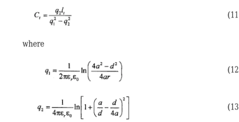
For the terminal capacitance of Ct, the same equation by which the capacitance between two wires of the bifilar type resistor can be calculated, is used. This was previously analyzed 6)and is given by
where
As shown in Figure 1, d is the terminal lead spacing, and ltis the length of the terminal leads.
The values listed in Table 1 were used to calculate the time (3)
(4)
(5)
(6)
(7)
(12)
(13) (2)
(11) (9)
(10) (1)
Table 1. Values of parameters used for calculating the time constant.
calculated to be 1.31 10-9s. To evaluate the uncertainty of this result, we analyzed the uncertainties of all values in Table 1.
3. Uncertainty analysis
With reference to the Guide to the Expression of Uncertainty in Measurement, the combined standard uncertainty of the time constant, uc( ), is obtained from (1), as
where c1,c2, , c9 are the sensitivity coefficients which are given by
3.1. Resistance of the wire; u(R)
The resistance of the quadrifilar reversed resistor was calibrated against the Quantized Hall Resistance (QHR). The QHR system realized at the NMIJ provides calibrations of 10 k resistance with a relative standard uncertainty of 0.03 / . Thus, the standard uncertainty of the resistance of the wire, u(R), was estimated to be 0.3 m .
3.2. Self-inductance of the wire; u(L)
As shown in Table 1, the relative permeability of the wire was assumed to be r = 1. Thus, from (2), the uncertainty in the derivation of the self-inductance of the wire, u(L), can be written as
where the sensitivity coefficients of c21and c22are
(24) Table 2. Values of resistance, inductance and capacitance of
the quadrifilar reversed resistor.
(17)
(18)
(14)
(19)
(20)
(21)
(22)
(23)
The uncertainty components that contribute to u(L) are restricted to the uncertainty of the folded length of the wire u(l) and the uncertainty of the wire radius u(r). The wires are folded on two supporting rods as shown in Figure 1, which can be moved for adjusting the strain of the wire. The distance between two supporting rods can easily be measured with an accuracy of mm, so that the folded length of l was estimated to be within mm. Also, the accuracy of the wire radius was estimated to be within m with reference to the manufacturer's specification. Assuming the rectangular distribution for each component, the standard uncertainties of the folded length u(l) and the wire radius u(r) were estimated to be 2.89 mm and 0.577 m, respectively. Consequently, from (24), the standard uncertainty of u(L) can be estimated to be 0.036 H.
3.3. Mutual inductance between adjacent wires ; u(M1)
From (3), the uncertainty in calculating the mutual inductance between adjacent wires, u(M1), can be written as
where c31and c32are
The uncertainty components that contribute to u(M1) are the uncertainty of the folded length of wire u(l) and the uncertainty of the wire spacing between adjacent wires u(c).
The estimation of u(l) is the same as in 3.2. The probability distribution of the wire spacing 2c was assumed to be rectangular with an interval of 20 5 mm. Thus, the standard uncertainty of u(c) was estimated to be 1.44 mm, and the standard uncertainty of u(M1) was calculated from (27) to be 0.011 H.
3.4. Mutual inductance between diagonally opposite wires;
u(M2)
From (4), the uncertainty of the mutual inductance between diagonally opposite wires, u(M2), is given by
where c41and c42are
As in (30), two components, that is, the uncertainty of the folded length u(l) which was estimated above, and the uncertainty of the wire spacing between diagonally opposite wires u(b) contribute to u(M2). It is supposed that the wire spacing 2b has a rectangular distribution of 28 7.1 mm because the relation of 2b= 2c exists as shown in Figure 1.
Thus, the standard uncertainty of u(b) was estimated to be 2.04 mm, and the standard uncertainty of u(M2) was calculated from (30) to be 0.011 H.
3.5. Capacitance between the wire and the outer shield; u(C0) The uncertainty equation with respect to the derivation of C0, which means the capacitance yielded between the total length of the wire and the shield, is given from (5), as
where the sensitivity coefficients using the values listed in Table 1 are
2
(33)
(34)
(35) (31)
(32)
(27)
(28)
(29) (26)
(30)
Moreover, from (8)-(10), the following equations can be derived:
where
Substituting (38)-(40) into (33), we obtain
length u(l), must be analyzed. Four of five have already been estimated as described above. Supposing that the dimension of the cylindrical shield was manufactured with the accuracy of 1 mm, then the standard uncertainty of u(a) in the assumption of rectangular distribution was estimated to be 0.577 mm. Thus, the standard uncertainty of u(C0) can be derived from (49) to be 0.252 pF.
3.6. Capacitance between adjacent wires; u(C1)
The uncertainty equation in the calculation of the total capacitance between adjacent wires, u(C1), can be derived from (6), as
and the sensitivity coefficients are
Substituting (38)-(40) into (50), we obtain
In (55), using the values estimated in the previous sections, the standard uncertainty of u(C1) was estimated to be 0.044 pF.
(38)
(40) (39)
(41)
(42)
(43)
(44)
(45)
(46)
(47)
(48)
(50)
(51)
(52)
(53)
(54)
(55) (37)
3.7. Capacitance between diagonally opposite wires; u(C2) From (7), the uncertainty of calculating the total capacitance between diagonally opposite wires, u(C2), is given by
where
Substituting (38)-(40) into (56), we obtain
3.8. Capacitance between the terminal leads; u(Ct)
From (11), the uncertainty with respect to the terminal capacitance, u(Ct) is given by
where the sensitivity coefficients are
Moreover, from (12) and (13), the following equations can be derived:
where
(66)
(67)
(68)
(69)
(70)
(72) (71) (57)
(58)
(59)
(60)
(61)
(62)
(63)
(64)
(65) (56)
Therefore, to estimate the uncertainty of the terminal capacitance u(Ct), the uncertainty due to the terminal lead spacing u(d) and the uncertainty due to the length of the terminal leads u(lt) need to be evaluated. In the resistor used in this analysis, however, the terminal leads are mostly shielded in order to minimize the terminal capacitance of Ct. Thus, the uncertainty of u(lt) means the imperfection of the shielding for the terminal leads. Because the unshielded length of the terminal leads was estimated to be lt= 5 5 mm, the standard uncertainty of u(lt) was calculated to be 2.89 mm, assuming the rectangular distribution for lt. Also, the spacing between the terminal leads was assumed to be d = 20 10 mm in the rectangular distribution, so the standard uncertainty of u(d) was estimated to be 5.77 mm. Consequently, the uncertainty of u(Ct) was evaluated using (73) to be 2.22 fF.
3.9. External capacitance added to the terminals; u(Ca)
By externally connecting a variable capacitor to the terminals, the time constant of the resistor is reduced almost to zero. The capacitance added to the terminals was measured by using a precision capacitance meter (AH 2500), which was calibrated against the NMIJ standard of capacitance. From the measurements, the standard uncertainty of u(Ca) was evaluated to be 0.58 fF.
Table 3 summarizes the results of the uncertainty analysis described above. Consequently, substituting these estimated values of uncertainties listed in Table 3 into (14), we determined the combined standard uncertainty uc( ) in the calculation of the time constant to be 6.0 10-10s.
This result means that the phase angle of the resistor can be determined with the standard uncertainty of 6.0 10-6 rad at an angular frequency of = 104rad/s. Therefore, with the quadrature bridge that can relate resistance to capacitance with the relative standard uncertainty of a few parts in 108[1], the loss angle of a capacitor is expected to be determined with
4. Conclusion
The time constant of the calculable AC resistor may be used as the standard of the capacitor loss angle. To derive a loss angle standard from the calculable time constant, we investigated the time constant of the quadrifilar reversed resistor and analyzed its calculation uncertainty. From the results, the standard uncertainty in calculating the time constant of the quadrifilar resistor can be estimated to be 6.0 10-10s. Thus, the standard of the capacitor loss angle in terms of the calculable time constant will be achieved with the uncertainty of the order of 1 in 106rad at = 104rad/s.
References
1) Y. Nakamura, M. Nakanishi and T. Endo, Measurement of frequency dependence of standard capacitors based on the QHR in the range between 1 kHz and 1.592 kHz IEEE Trans. Instrum. Meas.,vol. 50, pp. 290-293, 2001.
2) E. So and J. Shields, Losses in electrode surface film in gas dielectric capacitors, IEEE Trans. Instrum. Meas., vol.
(73)
4) J. Bohacek, Measurement of power factors of standard capacitors, IEEE Trans. Instrum. Meas., vol. 29, pp. 367- 369, 1980.
5) G. Ramm and H. Moser, From the calculable ac resistor to capacitor dissipation factor determination on the basis of time constant, IEEE Trans. Instrum. Meas.,vol. 50, pp.
286-289, 2001.
6) H. Fujiki, A. Domae and Y. Nakamura, Analysis of the
time constant for the bifilar calculable ac/dc resistors, in CPEM 2002 Dig.,pp. 344-345, 2002.
7) D. L. H. Gibbings, A design for resistors of calculable a.c./d.c. resistance ratio, Proc. Inst, Elec. Eng., vol. 110, pp. 335-347, 1963.
8) J. Bohacek, Metrologie Elektrickych Velicin (in Czech), Vydavatelstvi CVUT, Praha 1994.