Growth Effects of International Economic Integration

(1)

Growth Effects of International Economic Integration

著者 Hino Tomoko

出版者 Institute of Comparative Economic Studies, Hosei University

journal or

publication title

Journal of International Economic Studies

volume 25

page range 129‑148

year 2011‑03

URL http://doi.org/10.15002/00007899

(2)

Growth Effects of International Economic Integration

¹

Tomoko Hino

² November 19, 2010

Abstract

This paper quantitatively evaluates the influence of international risk sharing on economic growth by extending the analysis in Obstfeld (1994). However, whereas Obstfeld employs only data on the growth rate of consumption to calculate the returns on risky and risk-free assets, we include additional data on the total rates of return for risky assets and the deposit rates for risk-free assets. We also assume more realistic values for the degree of relative risk aversion and the elasticity of intertemporal substitution. Our calibrations indicate that a fully integrated financial market could significantly increase welfare.

(JEL classification: F21, G15, O16, O41)

1 Introduction

Does international financial integration enhance welfare? According to economic theory, when international asset trade expands and risk decreases, there is an improvement in international risk diversification. Investment in risky assets will then increase, along with returns. As a result, the increase in international asset trade will provide a welfare gain. The principal pur- pose of this paper is to provide an empirical analysis of this underlying economic theory.

In terms of related work, Obstfeld (1994) also considers the welfare gain from international asset trade where the mechanism linking international economic integration and growth is an attendant global portfolio shift from safe to riskier capital. On this basis, growth depends on the increase in risky capital. However, Obstfeld calibrates the gain from international financial integration by using only the growth rates of consumption in 64 countries. This is problematic given the reliance on consumption growth rates, the lack of currency of the data and the relatively small number of countries employed in the analysis.

The current paper extends this particular analysis by specifying total rate of return data for risky assets and deposit rates for risk-free assets, along with the consumption growth rates originally specified in Obstfeld (1994), to calibrate the gains from international financial integration. By using these data, the equilibria of risky and risk-free assets both pre- and post-economic integration are calculated, and the welfare gain from international asset trade are stud- ied. In addition, whereas Obstfeld allocates the 64 countries included across just eight regions,

1I am indebted to the constructive comments of an anonymous referee. The author would like to thank Akiko Tamura, Fumiki Yukawa, Kazutaka Takechi, Koichi Takeda, Nobusumi Sagara and especially Kenji Miyazaki for useful suggestions and welcome encouragement while undertaking this research. The author also acknowledges the helpful comments of Shingo Iokibe, Masaya Sakuragawa, Junmin Wan and other participants at meetings of the Japanese Economic Association, especially the 2008 spring meeting in Sendai. This research is financially supported by the Institute for

(3)

our study employs data from 124 countries (almost twice as many), and divides the data into 11 regions. Moreover, our analysis brings this important body of work up to date. Based on our analysis, we find that a welfare gain is brought about in every region through international financial integration, with calibration analysis showing that a fully integrated financial market could greatly increase welfare.

There are many studies on the effects of international risk sharing on economic growth.

For example, Jung (1986) investigates the causal relationship between financial development and economic growth by estimating Granger-causality between real GDP per capita and the ratio of CC³to M1 and M2 to GDP. Jung then concludes that financial development can be a cause of economic growth in developing countries. This appears to accord with the World Bank’s (1989) argument that the stimulation of investment is indispensable for economic growth. Moreover, without the presence of intermediate financial organizations, investment opportunities cannot be efficiently provided, and this hinders the accumulation of savings. In other work, Bencivenga and Smith (1991) consider the relationship between economic growth and the intermediate financial organizations that avoid risk, and Ziobrowski and Ziobrowski (1995) compare the performance of portfolios comprising only US assets and those consisting of assets from the USA, Japan and the UK. Their results show that portfolio performance is improved through internationally diversified investment and that higher returns can be obtained with the same level of risk by holding assets from three countries rather than one.

In yet other work on the impact of international financial integration on welfare, Baxter and Jermann (1997) consider human capital, and Imbs (2006) and Townsend and Ueda (2010) exploit fluctuations in GDP. Unfortunately, we are unable to draw fully on these important developments because of our intention to include many more countries in our analysis than any previous study⁴. As a result, there is inevitability some constraints on the types of data we have available.

The remainder of this paper is organized as follows. Section 2 presents the model. The results are presented in Section 3, and Section 4 concludes the paper. In an appendix, and in order to make a comparison with the seminal analysis in Obstfeld (1994), we provide calibrations using different parameters.

2 The Model

This section describes a model in which we consider two types of economies: a closed economy and a world economy.

A. Closed Economy

The household utility function⁵is defined as:

3CC: Currency in circulation outside the banking system.

4Baxter and Jermann (1997) employ data from four OECD countries, Imbs (2006) use data from 41 countries, and

(4)

where Etis expectation, C(t) is consumption at time t, εis the elasticity of intertemporal substitution, his a period prior to the economic decision, δis the subjective rate of time preference such that δ> 0, and R is the degree of relative risk aversion of households, such that R>0. In addition, f(x) is:

where U(t) is the constant relative risk aversion (CRRA) utility function.

Capital consists of risk-free and risky capital. The return on a risk-free asset is r(a constant) and the return on a risky asset is , such that > r. Let i(t) denote the real low-interest loan rate. If i(t) > r, risk-free capital is not in demand. If i(t) < r, it results in arbitrage profit from borrowing for investment in risk-free capital. If i(t)=r, it represents the equilibrium con- dition, and the risk-free asset consists of risk-free capital and borrowing. The real interest rate in the equilibrium is fixed.

Assets are defined as:

where B(t) is the risk-free asset and K(t) is the risky asset. Let i denote the risk-free rate of return and σis the standard deviation of returns on risky investments.

A change in assets is represented as follows:

The initial portfolio share of risky assets is:

Substituting ω(t) into Equation (2) yields:

where J(Wi) is the lifetime utility maximization level when wealth at time tequals W(t). Using Ito’s Lemma, the stochastic Bellman equation in continuous time resulting from maximizing U(t) in Equation (1) is:

(5)

From Equation (4), the first-order conditions are:

From Equation (1), maximized indirect lifetime utility is:

When we substitute J(W) into Equation (5), we obtain:

When we substitute J(W) into Equation (6), we obtain:

where ais a fixed number. Substituting into Equation (4) leads to:

where μis the expected utility.

(6)

B. Closed Economy Equilibrium

There are two different equilibrium cases. When , we have risky and risk-free

assets, where i=ris equilibrium. When , we have risky assets only, where i≠r.

When , the equilibrium rate of interest is .

From Equations (3) and (8), wealth accumulation is as follows:

From Equations (8) and (9), per capita consumption follows the stochastic process below:

The consumption growth rate is defined as:

From Equations (7) and (8), the consumption growth rate is:

The rate of growth is determined by:

Therefore, an increase in εpushes up the growth rate when i >δ. Equation (11) can be written as:

where is the risk-adjusted expected growth rate.

C. Growth Effects of International Economic Integration

We assume a multicountry world economy and a complete asset market. Let there by N countries, indexed by j=1,2,..., N. Each country has a preference such as shown in Equation (1).

Let Rjdenotes a relative risk-aversion coefficient, εjis the intertemporal substitution elasticity, and δjis the rate of time preference.

The symbol r is the rate of return on safe capital, which is common to all countries. The geometric diffusion process is:

(7)

where V^kis the cumulative value from investment of the capital, dtis a constant trend, dz(t) denotes a standard Wiener process, such that and denotes the instantaneous variance of returns. From Equation (12), the instantaneous correlation of the country-specific technology shocks is:

The symmetric covariance matrix of N×Nis:

where this covariance matrix has the inverse matrix.

The symbol 1is a column vector of N×1 with all entries equal to 1, is a column vector of N×1 the kth entry of which is k, and ωωj is a column vector of N×1 the kth entry of which is the demand for country k’s risky capital by a resident of country j.

The weight of risky assets is:

where i*is the world real interest rate.

The rule for investment decision depends on the investment trust theory of Merton (1971). The portfolio weight for the resulting mutual fund is:

where θθis the N×1 vector. The “prime”(’) is the matrix transposition. The portfolio weight is constant. Therefore, a single risky asset in the world with mean return is:

The return variance of mutual fund annual return is:

and the share of the fund in global wealth is:

Next, we consider the equilibrium. A closed economy shifts to an open economy through international financial integration. All types of capital are unboundedly changeable, but the relative prices of assets are fixed at 1. Instead, available quantities are variable (i*, and ΩΩ are given). Here, we can stimulate investments where the asset share is greater than 1 through a global mutual fund of risky assets. Country j’s mean growth rate is:

(8)

3 Calibration

This section is devoted to an example illustrating the gains from international financial integration. The example is based on actual consumption growth data, deposit rates and total rates of return. We calibrate two types of gain: stochastic and deterministic.

The structure of this section is as follows. To begin, we calculate the means and standard deviations of the consumption growth rates. We then calculate the returns of the risky and risk-free assets and the initial portfolio shares of risky assets and the standard deviations of returns on risky investment. Finally, we calculate the welfare gains from financial integration.

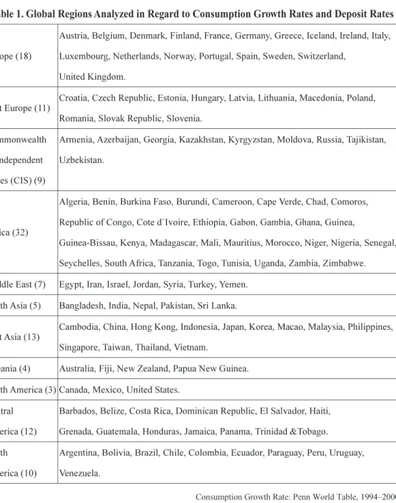
Table 1. Global Regions Analyzed in Regard to Consumption Growth Rates and Deposit Rates

(9)

Additionally, in the appendix, in order to make a comparison with the analyses of Obstfeld (1994), we perform calibrations in the same way as Obstfeld’s. We calculate the welfare gains resulting from financial integration by using only the consumption growth rate fixed under the assumption of an equity premium of 4 percent and by setting the same parameters (R, εand δ) with Obstfeld’s. We have also performed calibrations using a similar set of parameters to those of this section. Therefore, we can validly compare the results of analyses in this section with those presented in the appendix.

Consumption growth rates between 1994 and 2000 are taken from the Penn World Table⁶. We use the Consumer Price Index (CPI) data for calculating the real consumption growth rates. The CPI data are drawn from the International Financial Statistics (IFS) published by the International Monetary Fund (IMF). As illustrated in Table 1, we then categorize the 124 countries for which data are available into 11 regions, namely, Europe, East Europe, Commonwealth of Independent States (CIS), Africa, Middle East, South Asia, East Asia, Oceania, North America, Central America and South America.

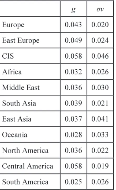
Table 2 provides the means and standard deviations of the consumption growth rates.

From Equation (10), consumption per capita is:

where v(t) is an independently and identically distributed random variable, such that and The mean consumption growth rates are relatively high for the CIS (0.058), Central America (0.058) and Eastern Europe (0.049), whereas those of Oceania (0.028) and South America (0.025) are relatively low. Likewise, the standard

Table 2. Mean and Standard Deviations of Consumption Growth Rates

(10)

deviations of the consumption growth rates of the CIS (0.046) and East Asia (0.041) are relatively high, but relatively low for Europe (0.02) and Central America (0.019).

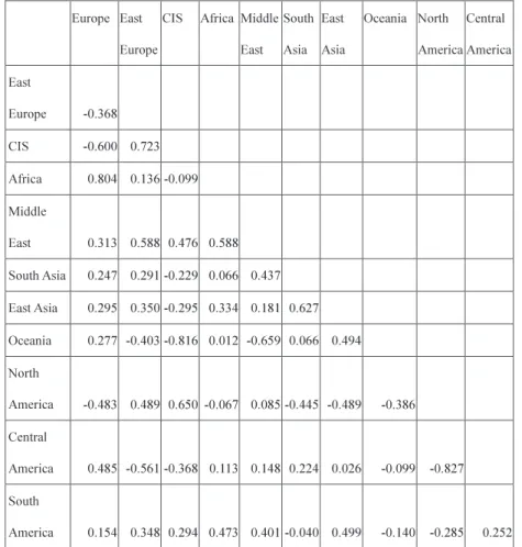
Table 3 details the correlation coefficients of the regional per capita consumption growth rates. Perfect risk pooling, which is the goal of financial integration, would occur if all entries in the correlation matrix were equal to one. As shown, the correlation coefficient between Africa and Europe is very high at 0.804.

Table 3. Correlation Coefficients of Regional Per Capita Consumption Growth Rates

(11)

Table 5 provides the returns on risky assets ( ) and risk-free assets (i) and the equity risk premium. We use deposit rates from the IFS to represent the profit on risk-free assets and the total rates of return from the World Federation of Exchanges for 1995-2000 to denote the profit on risky assets (we remove the 1997 data for East Asia because of the abnormality of the data given the influence of the Asian currency crisis). The symbols iand are converted to real rates using the CPI (from the IFS). As is only collected from a limited number of

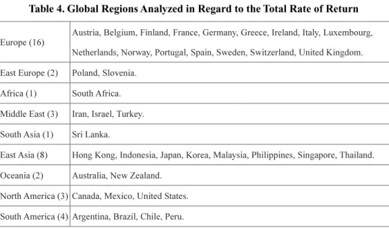
Table 4. Global Regions Analyzed in Regard to the Total Rate of Return

Table 5. Real Deposit Rates, Real Total Rates of Return and Equity Premiums

(12)

from Eastern Europe and South America for the CIS and Central American total rates of return, respectively. Although iis theoretically positive for CIS and Africa, negative values are found in the actual data. This is because inflation exerts an impact at the time of conversion to real rates using the CPI. However, as iis greater than (see Table 5), we use the negative values from the data.

In general, the values of iare relatively large in Central America (0.033), the Middle East (0.032) and East Asia (0.03), and is especially large in the Middle East (0.56) and Europe (0.217). The smallest value of iis in the CIS (–0.039) and the smallest is in Africa (0.037).

Lastly, the equity premium is relatively large in the Middle East (0.527) and Europe (0.203) and relatively small in East Asia (0.014) and Central America (0.018).

Table A1 in the appendix details the calculation of the values of iusing the data on consumption growth rates and the set of parameters from Obstfeld (1994).

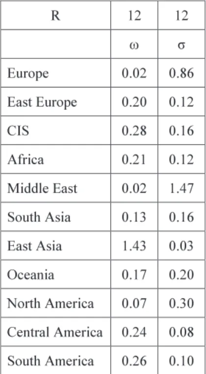
Table 6 provides the initial portfolio shares of risky assets (ω) and standard deviations of returns on risky investment (σ) calculated using the equity premiums in Table 5. We assume that Ris 12, although Obstfeld (1994) assumes that Ris 18⁷. However, as Obstfeld also dis- cusses, the value of R=18 is unrealistically large and, for this reason, we have assumed R=12.

Also, R and λhave a positive correlation when only R changes and the other conditions remain the same.

The initial portfolio shares of risky assets are calculated using the equation:

Table 6. Initial Portfolio Shares of Risky Assets and Standard Deviations of the Annual Return to Risky Investments

(13)

The standard deviations of the annual return to risky investment are calculated using:

Here, Equation (17) can be changed to As a result, the deviation of the return on a risky investment has a positive correlation with the equity premium and a negative correlation with R. That is, the greater the degree of risk aversion, the lower the demand for risky assets. In addition, the greater the risk involved in risky assets, the greater the risk premium required.

In Table 6, the share of risky assets for East Asia is greater than one, indicating a short position. This is because the equity premium is extremely small in comparison with the variance of consumption growth rates. In this situation, the value of the standard deviation of the annual return on risky investment is low, and ωis large. To be precise, as the risk involved in risky assets is low, the demand for risky assets increases along with the share of these assets.

It may be interesting to calculate the relationship between ωand the share of risky assets using actual data. However, it is difficult to undertake this calculation as we typically lack this information for many developing countries. Moreover, it is not easy to compare the data in developed countries even when available. The definition of households differs from country to country⁸. For example, sole proprietorships are included with households in Japan but with corporations in France, Germany and the UK.

Despite these differences, we attempt to calculate the share of risky assets in Japan. We do this by using the flow of funds accounts from the Bank of Japan between 1994 and 2000.

This indicates that the share of risky assets averages 6 percent. As our calibration with R=18 and R=12 indicates a respective average of 5 and 3 percent, it would appear that there is little difference between ωand the share of risky assets suggested by actual data, at least in Japan.

We also discuss the situation in developing countries, for which there are several previous studies. According to Rajan and Zingales (2001) and Levine (1997, 2004), developing countries exhibit relatively more risk aversion than developed countries because wealth in developing countries is generally lower. In addition, it is generally argued that financial markets do not work well in developing countries. For this reason, banks dominate the markets. As show in Table 6, regions composed of developing countries generally have higher values of ω. We surmise that the gap may be the result of other macroeconomic factors. However, this is beyond the focus of our analysis.

In Table A2 in the appendix, ωand σare calculated for the cases where -i=0.04 (from Equations (17) and (18)) with an Rvalue of either 12 or 18.

(14)

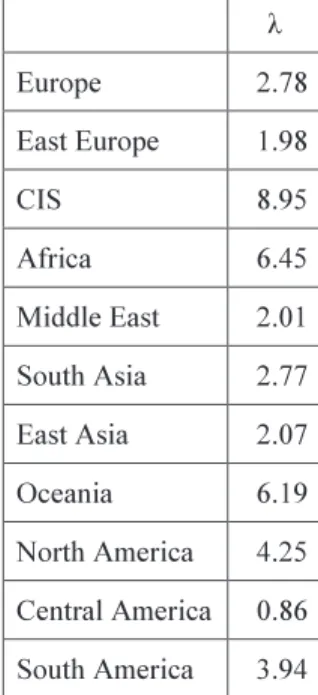
Table 7 details the welfare gains from financial integration. We first calculated the value of i*, *, σ*, ω* and g*post-financial integration. As investment in the region with the highest value of iwill presumably increase because of financial integration, the value of ifor the region with the highest pre-financial integration value becomes the post-interest rate (i*).

The values *, σ*, ω* and g* are calculated using Equations (13), (14), (15) and (16), respectively.

As shown, ω* is greater than one, indicating that short selling is taking place. When actual data are used, the variance of the post-financial integration return to risky investment (0.05) is low in comparison with the post-financial integration equity premium (0.052). This indicates risky assets with low risk and high returns and, of course, the share of risky assets increases.

We also assume that εis 0.8. Although Obstfeld (1994) assumes ε= 1.1⁹, according to both Campbell and Mankiw (1989) and Attanasio and Weber (1993), εis less than 1. For this reason, we employ a value of 0.8. In addition, when other conditions are the same and only ε changes, εand λhave a positive correlation and, when other conditions are the same and only δchanges, δand λhave a negative correlation.

From Equations (8) and (10), the welfare gain from financial integration is:

As a result, welfare gains from financial integration are achieved in all regions with an average gain of 3.84. As in Obstfeld (1994), σ* is lower than its pre-financial integration

Table 7. Gains from International Financial Integration

(15)

value in all regions, whereas ω*and g*are higher. That is to say, because financial integration risk is shared, the risk involved in risky assets decreases, and thus investment in risky assets yields higher returns and welfare gains result.

As shown, welfare gains become larger when consumption growth rates and the returns on risk-free assets for both pre- and post-financial integration vary widely (CIS and Africa).

With regard to Central America, as the region has the highest value of ibefore financial integration, a welfare gain is still achieved even though the value of i has not changed. This is because the consumption growth rate, which was 5.8 percent before financial integration, increased to 9.1 percent (g*) after integration.

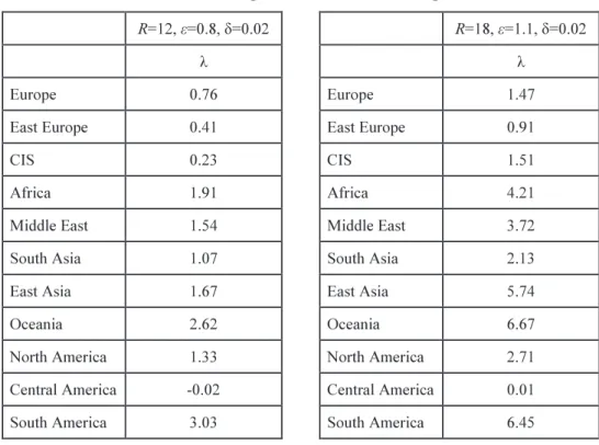
Table A3 in the appendix provides the welfare gains calculated using and i obtained through calibration and the set of parameters in Obstfeld (1994).

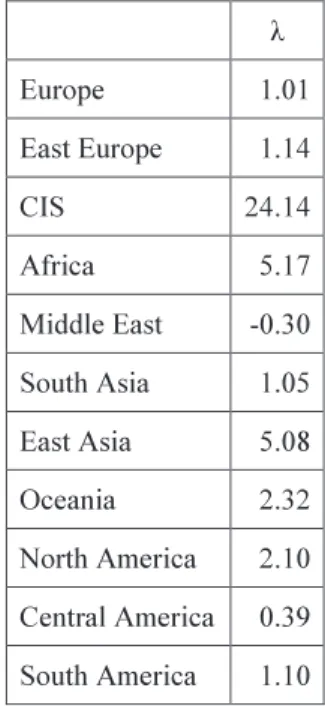
In Table 8, we calibrate the welfare gains where the gain from a pure international technology transfer is measured by the gains from switching deterministic technologies. These are the gains obtained only from the change in the rate of return associated with financial integration. Optimum consumption before f inancial integration in the deterministic model is , where the rate of return is ω +(1–ω)i. Following financial integration, optimum consumption is , and the rate of return is ω *+(1–ω)i*. The gains from switching deterministic technologies are then:

Table 8. Gains from Switching Deterministic Technologies

(16)

In the deterministic case, only ωand changes to and ibefore and after financial integration have an impact on welfare gains. As shown, CIS has the largest λ, given that the change in ibefore and after financial integration is now 0.072; a value far larger than that given earli- er in Table 7. Although the value of λfor East Asia is also larger than in Table 7, it is only because the value of ωfor East Asia is relatively large at 1.43. The Middle East has the only negative value. This is because the value of for the Middle East before financial integration is extremely high and decreases 47.5 percent as a result of financial integration. In the deterministic case, given that only the changes in and i have an impact on welfare gain, the decrease in cannot be offset and the gain is therefore negative.

In Table A4 in the appendix the welfare gains for the deterministic case are calculated using and iand a similar calibration to Obstfeld (1994).

4 Conclusion

In this paper, we calculated the welfare gains from international asset trade using consumption growth rates, total rates of return and deposit rates. We find that every region yields welfare gains from international asset trade and that the average welfare gain among all regions is 3.84. The results also indicate that the welfare gain becomes larger in regions with fewer risk-free assets.

In terms of limitations, the analysis in this paper employs total rate of return data for risky assets and deposit rates for risk-free assets. It is then possible that the analysis could be improved by using better quality data.

On the other hand, it is obvious that this paper is not giving a clear explanation of the cause of global financial crisis which happened in 2008. The author thinks that the global financial crisis can be attributed to the fact that crucial global imbalances was brought about by excessive capital inflow to the United States. However, imbalanced factors are not consid- ered in this paper. It may be possible to analyze this phenomenon by studying the factors of this imbalance. We should take this issue as the next step to overcome.

Appendix

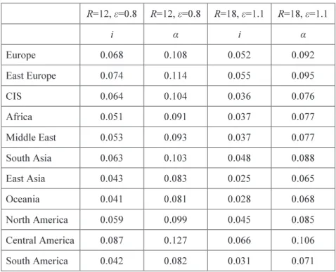
In order to compare our work with the analysis in Obstfeld (1994), we perform calibrations in a similar manner in this appendix and calculate the welfare gains with an assumption of a 4 percent equity premium for all regions. Further, because Obstfeld assumes R=18, to compare Obstfeld’s calibrations with those in the current paper, we calculate the welfare gains for when R=12 and 18.

The appendix is organized as follows. First, Table A1 presents the rates of return on the risk-free and risky assets. Table A2 then provides the standard deviations of the initial portfolio shares of risky assets and the returns on risky assets. In Table A3, welfare gains are calculated when the values for R, εand δare as in Obstfeld (1994) and when these values are the

(17)

gains in the deterministic case for identical conditions to those in Table A3.

In Table A1, the returns on the risk-free assets (i) are calculated using consumption growth rates (see Table 2). Converting Equation (11) through substituting yields:

The return on risk-free assets can then be calculated using this equation. The value of can be calculated by assuming −i = 0.04.

As shown, although we assume an equity premium of 4 percent, half of the equity premiums obtained from actual data are lower than 4 percent (see Table 5). However, as there are some regions with exceedingly high values, the average equity premium is 10.5 percent. The values for the risk-free assets in Table A1 are also greater than the actual data in all regions (see Table 5), with an average of 0.046. The returns on the risk-free assets in Table A1 also have a negative correlation with the variance of the consumption growth rates and a positive correlation with the consumption growth rates themselves. For instance, although the average consumption growth rate for the CIS and Central America are nearly the same, the variance is 4.6 percent for CIS and 1.9 percent for Central America. For this reason, differences of more than 2 percent in the return on risk-free assets accrue. That is, as the variance of the consumption growth rate and risk increase, the returns on the risk-free assets decrease.

Table A1. Risk-free and Risky Rates of Return where -i=0.04

(18)

In Table A2, ω ^andσ are calculated where -i=0.04 (from Equations (17) and (18)) with an Rvalue of either 12 or 18. The result, which accords with that in Obstfeld (1994), is that the share of risky investments decreases in regions where the variance in consumption growth rates is low. That is, although returns are high when consumption growth rates are sta- ble, highly risky investments are avoided. Examination of Table 6 and Table A2 indicates that in both situations when Ris large the values of the standard deviation of the annual return to risky investment is small. This means that the higher the degree of risk aversion, the greater the desire to avoid risky assets.

In Table A3, the welfare gains from financial integration are shown, calculated using only the consumption growth rate, an equity premium of 4 percent and the set of parameters in Obstfeld (1994). Note that Obstfeld assumes R=18, ε=1.1 and δ=0.02. A comparison of the right-hand side of the table with the results in Obstfeld indicates that the welfare gains here are considerably larger. This is because ω*increases as the value of *-i*is larger than σ*;

as a result, g* is at least twice as high as the value in Obstfeld. That is, returns increase because of an increase in the share of risky assets resulting from a lower risk in proportion to the returns obtained from risky assets, and consumption growth rates increase as a result.

A comparison of Table 7 with the left-hand side of Table A3 shows that the welfare gain in Table 7 is larger. This is because the difference in equity premiums before and after financial integration is greater where actual data are used, given the value of iis low and the value of is high. Although the pre-financial integration equity premium is 4 percent in Table A3, the average regional equity premium employed in Table 7 is 10.5 percent.

Table A2. Initial Portfolio Shares of Risky Assets and Standard Deviations of the Annual Return to Risky Investments where -i=0.04

(19)

Table A3. Gains from International Financial Integration where -i=0.04

Table A4. Gains from Switching Deterministic Technologies where -i=0.04

(20)

In Table A4, we show the results where the welfare gains for the deterministic case are calculated using only the consumption growth rate data. The total amount of welfare gains is smaller than in Table A3. This result accords with that in Obstfeld (1994). This is because, in the deterministic case, only changes in and ihave an impact on the welfare gains. In addition, we can see that the total amount of welfare gain is larger in Table 8 (using actual data for both and i) than in Table A4. This is because, when actual data are used, there are regions where asset returns change markedly because of financial integration. We can also see that the total amount of welfare gains is greater for R=18 than for R=12 because both Rand ε are higher in the former.

References

Attanasio, O. P. and G. Weber, (1993), Consumption Growth, the Interest Rate and Aggregation. Review of Economic Studies60(3), 631-49.

Baxter, M. , and U. J. Jermann, (1997), The International Diversification Puzzle is Worse than You Think. The American Economic Review87(1), 170-80.

Bencivenga, V. R. , and B. D. Smith, (1991), Financial Intermediation and Endogenous Growth. Review of Economic Studies58(2), 195-209.

Campbell, J. Y. and N. G. Mankiw, (1989), Consumption, Income and Interest Rates:

Reinterpreting the Time Series Evidence, NBER Macroeconomic Annual 1989 4, 185–216.

Epstein, L. G. and S. E. Zin, (1989), Substitution, Risk Aversion and the Temporal Behavior of Consumption and Asset Returns: A Theoretical Framework. Econometrica57(4), 937-69.

Imbs, J. (2006), The Real Effects of Financial Integration. Journal of International Economics68(2), 296-324.

Jung, W. (1986), Financial Development and Economic Growth: International Evidence.

Economic Development and Cultural Change, January.

Levine, R. (1997), Financial Development and Economic Growth: Views and Agenda.

Journal of Economic LiteratureXXXV, 688-726.

Levine, R.(2004), Finance and Growth: Theory and Evidence. NBER Working Paper Series 10766.

Merton, R. C. (1971), Optimum Consumption and Portfolio Rules in a Continuous-Time Model. Journal of Economic Theory3(4), 373-413.

Obstfeld, M. (1994), Risk-Taking, Global Diversification, and Growth. The American Economic Review84(5), 1310-29.

Rajan, R. G. and L. Zingales, (2001), Financial System, Industrial Structure, and Growth.

Oxford Review of Economic Policy17(4), 467-82.

Bank of Japan, (2000), Points on International Comparison of the Flow of Funds Accounts.

http://www.boj.or.jp/

Summers, R. and A. Heston, (1991), The Penn World Table (Mark 5): An Expanded Set of International Comparisons, 1950-1988. Quarterly Journal of Economics106(2), 327-68.

Townsend, R. M. and K. Ueda, (2010), Welfare Gains from Financial Liberalization.

International Economic Review51(3), 553-597.

Weil, P. (1989), The Equity Premium Puzzle and the Risk-Free Rate Puzzle. Journal of Monetary Economics24(3), 401-21.

(21)

105(1), 29-42.

World Bank,(1989), World Development Report 1989. Oxford University Press.

Ziobrowski, B. J. and A. J. Ziobrowski, (1995), Exchange rate risk and internationally diver- sified portfolios. Journal of International Money and Finance14(1), 65-81.