M
ul t i - s ec t or al val ue c hai n i n a bi l at er al
gener al equi l i br i um
著者
N
akano Sat os hi , N
i s hi m
ur a Kaz uhi ko, Ki m
J i young
権利
Copyr i ght s 日本貿易振興機構(ジェトロ)アジア
経済研究所 / I ns t i t ut e of D
evel opi ng
Ec onom
i es , J apan Ext er nal Tr ade O
r gani z at i on
( I D
E- J ETRO
) ht t p: / / w
w
w
. i de. go. j p
j our nal or
publ i c at i on t i t l e
I D
E D
i s c us s i on Paper
vol um
e
691
year
2018- 02
INSTITUTE OF DEVELOPING ECONOMIES
IDE Discussion Papers are preliminary materials circulated to stimulate discussions and critical comments
Keywords: Linked Input–Output Tables, Information and Communications Technology,
Tracing Elasticities
JEL classification: C67, D57, D83, F19
*Research Fellow, Global Value Chains Studies Group, Inter-disciplinary Studies Center, IDE ([email protected])
IDE DISCUSSION PAPER No. 691
Multi-Sectoral Value Chain in a Bilateral
General Equilibrium
Satoshi NAKANO, Kazuhiko
NISHIMURA and Jiyoung KIM*
February 2018
Abstract
The information and communication technology (ICT) is a key engine of economic
growth. In this paper, we examine the impact of ICT innovation using a multifactor
constant elasticity of substitution (CES) general equilibrium model. Innovation not only
leads to productivity growth and thus influence prices, it also changes output and trade
patterns, and welfare. To examine trade values, we construct a bilateral multifactor CES
general equilibrium model between Japan and the Republic of Korea using linked
input–output tables. We estimate elasticities of substitution and productivity growths of
The Institute of Developing Economies (IDE) is a semigovernmental,
nonpartisan, nonprofit research institute, founded in 1958. The Institute
merged with the Japan External Trade Organization (JETRO) on July 1, 1998.
The Institute conducts basic and comprehensive studies on economic and
related affairs in all developing countries and regions, including Asia, the
Middle East, Africa, Latin America, Oceania, and Eastern Europe.
The views expressed in this publication are those of the author(s). Publication does
not imply endorsement by the Institute of Developing Economies of any of the views
expressed within.
INSTITUTE OF DEVELOPING ECONOMIES (IDE), JETRO
3-2-2, WAKABA, MIHAMA-KU, CHIBA-SHI
CHIBA 261-8545, JAPAN
Multi-Sectoral Value Chain in a Bilateral General Equilibrium
Jiyoung Kim*a, Satoshi Nakanob, Kazuhiko Nishimurac
aInstitute of Developing Economies
bThe Japan Institute for Labour Policy and Training cNihon Fukushi Univerisity, Faculty of Economics
Abstract
The information and communication technology (ICT) is a key engine of economic growth. In this paper, we examine the impact of ICT innovation using a multifactor constant elas-ticity of substitution (CES) general equilibrium model. Innovation not only leads to pro-ductivity growth and thus inluence prices, it also changes output and trade patterns, and welfare. To examine trade values, we construct a bilateral multifactor CES general equilib-rium model between Japan and the Republic of Korea using linked input–output tables. We estimate elasticities of substitution and productivity growths of the ICT sectors, to assess the efects of ICT improvement on the two countries.
Keywords: Linked Input–Output Tables, Information and Communications Technology, Tracing Elasticities
1. Introduction
Recently, Kim et al. (2017) developed a bilateral multifactor constant elasticity of substi-tution (CES) general equilibrium model with state-replicating Armington elasticities; each elasticity of substitution between foreign and domestic commodities is measured by a two-point calibration, such that the Armington aggregator can replicate the two temporally distant observations of market shares and prices. This study integrates the domestic pro-duction of two countries, Japan and the Republic of Korea, with bilateral trade models and constructs a bilateral general equilibrium model.
In this paper, we examine the efect of the information and communication technology (ICT) sector on economic growth using a bilateral multifactor CES general equilibrium model. The ICT sector has become the leading sector of the global economy. According to
∗Corresponding Author.
OECD (2017), value added for the ICT sector and sub-sectors stood at 5.4% of all OECD countries in 2015. Among 31 countries, the Republic of Korea ranked irst with 10.3%. More speciically, ICT manufacturing accounted for 7.2%, telecommunications for 1.3%, and information technology (IT) and other information services for 1.9%. Japan ranked sixth with 6.0%, of which 1.7% came from ICT manufacturing, 1.8% from telecommunications, and 2.4% from IT and other information services. Moreover, OECD (2017) demonstrated a constant rise in the spread of ICT infrastructure and a growing demand for ICT goods on trade.
Some empirical studies have shown ICT’s importance in economic growth. Farhadi et al. (2012) found that ICT use had a signiicant efect on economic growth by using panel data of 159 sample countries. Despite numerous studies showing the important role played by the ICT sector, evidence of its contribution to economic growth in developing countries is lacking. For example, the empirical results of Lee et al. (2005) indicate that ICT investments have been contributing to an improvement in economic growth in many developed and newly industrialized economies. However, it was not signiicant in developing countries, such as China. Zuhdi et al. (2012) showed the ICT sector played an important role in changing the structure of Japan’s economy, but did not have a signiicant efect in Indonesia.
We build a bilateral multifactor CES general equilibrium model between Japan and the Republic of Korea to bridge this research gap. Although evidence of the ICT sector’s importance in growth for developing countries is still scarce, some studies have been able to show this in Japan and Korea. (Jorgenson and Motohashi (2005), Kanamori and Motohisa (2007), Zuhdi et al. (2012), Jung et al. (2013), Ju (2014)).
2. Methodology
2.1. Two-point calibration of the CES function
Let us begin with a two-input production function with constant CES, as follows:
z =F (x, y) =θ α1/σx1−1/σ
+β1/σy1−1/σ1/(1−1/σ) (1)
where x and y denote the physical level of the two inputs and z denotes the output in
physical units. As for the parameters, σ > 0denotes the elasticity of substitution, whereas
α >0and β >0 denote the share parameters whereα+β = 1. The level of productivity is
Notice that the following function represents the (dual) unit cost that corresponds to the production function (1):
r =G(p, q) = θ−1
αp1−σ
+βq1−σ1/(1−σ)
(2)
wherepand q denote the prices for the irst and second factor, respectively, whilerdenotes
the output price (or, the unit cost of the output). We can verify that (2) and (1) are dual as follows:
First, the isoquant of (1) must be tangent to the price ratio, that is:
∂y ∂x
z
=−∂z
∂x/ ∂z ∂y =−
α β y x 1/σ
=−p
q
Thus, the cost share ratiob/a(i.e., the cost share of the second inputb= pxqy+qy with respect
to the irst inputa = pxpx+qy) would be
b a = qy px = β α q p
1−σ
(3)
Alternatively, since (2) is homogeneous in degree one, Euler’s rule implies that
r = ∂G
∂pp+ ∂G
∂qq =xp+yq=θ
−1 α r p σ
p+θ−1
β r q σ q
and we can obtain the cost share ratio that is identical to (3) through (2) as well.
Now, let us look at the cost shares of the inputs (a0, b0;a1, b1), and the prices of inputs
and outputs (p0, q0, r0;p1, q1, r1) for two diferent periods, where we indicate periods by
subscript 0 (reference) and 1 (current). One can verify, with reference to (3), that the following parameters can be obtained from the observables, i.e.,
1−σ = lna
1/a0−lnb1/b0
lnp1/p0−lnq1/q0 (4)
lnα= lna0−(1−σ) lnp0/r0 = lna1−(1−σ) lnp1/r1 (5)
lnβ = lnb0−(1−σ) lnq0/r0 = lnb1−(1−σ) lnq1/r1 (6)
θ0 =α p0/r01−σ
+β q0/r01−σ
(7)
θ1 =α p1/r11−σ
+β q1/r11−σ
(8)
satisfy the inputs and outputs of the CES unit cost function (2) for the two periods,
r0 = (θ0)−1
α(p0)1−σ
+β(q0)1−σ1/(1−σ)
(9)
r1 = (θ1)−1
α(p1)1−σ
+β(q1)1−σ1/(1−σ)
(10)
Thus, we call the parameters obtained through (4–8) as state replicating and the procedure, two-point calibration.
Notice that (1) becomes an aggregator function ifθ is constant. In that case, the
state-replicating aggregator function can be two-point calibrated by (4–6) using the observed cost shares and prices of the inputs for two periods, i.e., (a0, b0;a1, b1) and (p0, q0;p1, q1), while
the two output (aggregated) prices (r0, r1)are evaluated using the following formulae:
r0 = α(p0)1−σ
+β(q0)1−σ1/(1−σ)
(11)
r1 = α(p1)1−σ
+β(q1)1−σ1/(1−σ)
(12)
Alternatively, when the output price is observed but one of the input prices (say, for the second input) is not observed, we may still calibrate the parameters as follows:
1−σ = lna
1/a0
lnp1/p0−lnr1/r0 (13)
lnα= lna0−(1−σ) lnp0/r0 = lna1−(1−σ) lnp1/r1 (14)
lnβ = ln(1−α) (15)
Note that in this case, the price of the second factor(q0, q1)can be evaluated as follows:
q0 =
(r0)1−σ
−α(p0)1−σ
β
1/(1−σ)
, q1 =
(r1)1−σ
−α(p1)1−σ
β
1/(1−σ)
2.2. Multifactor CES elasticity of substitution
A multifactor CES unit cost function is of the form
p=θ−1
λ0(p0)1−σ
+λ1(p1)1−σ
+· · ·+λN(pN)1
−σ1/(1−σ)
(16)
wherep0, p1,· · · , pN denote the input prices, pdenotes the output price, and λ0, λ1,· · · , λN are the share parameters where PN
but we can estimate them using regression, as follows: Applying Shepard’s lemma for (16) yields the following:
si =
∂p ∂pi
pi
p =λi
pi
θp
1−σ
(17)
By taking the log on both sides we have:
lnsi = lnλi−(1−σ) lnθ+ (1−σ) lnpi/p (18)
Since factor cost shares are observable for two periods (s0
i, s1i) for all inputs i= 0,1,· · · , N in a set of linked input–output tables, the following two equations must hold:
lns0i = lnλi−(1−σ) lnθ0+ (1−σ) lnp0i/p0
lns1i = lnλi−(1−σ) lnθ1+ (1−σ) lnp1i/p1
Subtracting, we have:
lns1
i/s0i =−(1−σ) lnθ1/θ0+ lnp1/p0
+ (1−σ) lnp1
i/p0i
∆ lnsi =−(1−σ) (∆ lnθ+ ∆ lnp) + (1−σ)∆ lnpi (19)
That is, the multifactor CES elasticity of substitution σ can be estimated by the slope of
the simple regression line between the growth of cost shares and the growth of factor prices. Moreover, the intercept of the regression line provides an estimate of productivity growth
lnθ1/θ0, given the estimate of its slope (1−σ).
3. Measurement
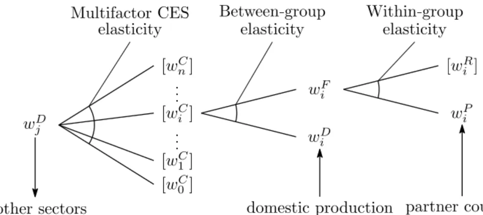
The substitution structure of the bilateral general equilibrium model is illustrated in Figure 1. We measure multifactor (intermediate) CES elasticity of substitution by using the 1995–2000–2005 linked input–output tables for both Japan (MIAC, 2011) and Korea (BOK, 2009), choosing 2000 as the reference and 2005 as the current period. For the measurement of Athe rmington elasticities, we use the six-digit HS trade data of the UN Comtrade database (Comtrade, 2017) that covers 6,376 goods converted into the linked input–output sector classiication, to obtain the market share of the partner country with respect to the rest of the world (ROW) for the corresponding two periods. In this study, the state-replicating Armington elasticities are measured in a two-stage nested structure.
Figure 1: Substitution structure of the bilateral general equilibrium model.
For each traded good, we irst calibrate the within-group elasticity that replicates the observed partner–ROW market shares with regard to price changes of the partner country-made commodity, and that of the compound commodity (i.e., compound of the partner’s and the ROW’s commodities) which we monitor as the foreign commodity, for the two periods concerned. We then calibrate the between-group elasticity that replicates the observed domestic–foreign market shares with regard to price changes of the corresponding factor prices for the two periods. Finally, we measure the multifactor CES elasticity of substitution through ia regression.
3.1. Armington Elasticities 3.1.1. Within-group Elasticities
The within-group aggregator is the two-input CES function that compounds the com-modity of one kind imported from the partner country and that from the ROW. For each commodity j, the dual aggregator function can be written as follows:
wjF = αj(wjP)1
−σj
+βj(wRj )(1
−σj)1/(1−σj)
≡Vj wPj , wjR
(20)
where, wF
j , wPj , wjR denote prices of foreign, partner, and ROW commodity j, respectively. The parameters are calibrated by (13–15) using the observed values of wF
j , wPj and market shares sP
0
10
20
30
40
Frequency
−2 0 2 4 6 8
Log Abs Elasticity
0
10
20
30
40
Frequency
−2 −1 0 1 2 3
Log Abs Elasticty
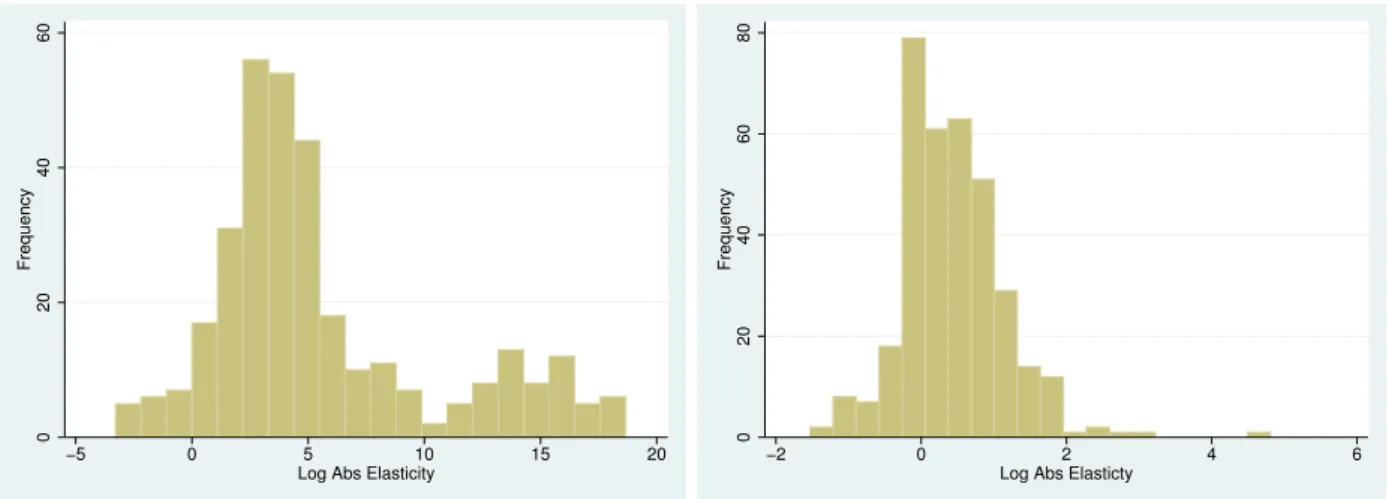
Figure 2: Histogram of calibrated between-group elasticities in log-absolute values for Japan (left) and Korea (right).
0
20
40
60
Frequency
−5 0 5 10 15 20
Log Abs Elasticity
0
20
40
60
80
Frequency
−2 0 2 4 6
Log Abs Elasticty
Figure 3: Histogram of calibrated within-group elasticities in log-absolute values for Japan (left) and Korea (right).
3.1.2. Between-group Elasticities
The between-group aggregator is the two-input CES function that compounds the for-eign (imported) and domestically produced commodities. For each commodity j, the dual
aggregator function can be written as follows:
wCj = αj(wDj )1
−σ
+βj(wFj )(1
−σj)1/(1−σj)
≡Uj wDj , wjF
(21)
wherewC
j , wjD, wjF denote the prices of the compound, domestic, and foreign commodity j, respectively. The parameters are calibrated by (4–6) using the observed values of wD
j , wjF and market shares sD
j , sFj for the two periods. In Figure 2, we display the histogram of the
−1
0
1
2
3
4
sigma
0 100 200 300 400 sector
−1
0
1
2
3
4
sigma
0 .2 .4 .6 .8 1
pval slope
Figure 4: Estimated multifactor CES elasticities and their statistical signiicance, for Japan.
calibrated between-group elasticities of 395 commodities for Japan and 350 commodities for Korea. Overall, the calibrated within-group elasticities are very large, which means that the domestic and foreign commodities are (almost complete) substitutes. Note that the log-absolute values (with base of 10) are used to display the elasticities.
3.2. Multifactor CES Elasticities
We estimate the multifactor CES elasticities for all production sectors according to the regression equation (19). For the explanatory variables in the regression, we use the growth of compound factor prices i.e., ∆ lnwC
i which we calculate by using the between-group ag-gregator (21) for each commodity. In Figure 4, we display the estimated multifactor CES elasticity of substitution for Japan (395 sectors). The corresponding statistical signiicances are indicated in the right-hand side igure. In Figure 5, we display the estimated multi-factor CES elasticity of substitution for Korea (380 sectors). The corresponding statistical signiicances are indicated in the right-hand side igure.
Figure 6 shows the productivity growth ∆ lnθj (or, total factor productivity growth TFPg) for all j sectors, which can be estimated from the intercept of the regression line of
(19), for Japan. On the right-hand side of the igure, we display the corresponding statistical signiicances of the intercept and the slope of the regression line. Similarly, in Figure 7 we display the productivity growth ∆ lnθj (or, total factor productivity growth TFPg) for all
0
1
2
3
sigma
0 100 200 300 400
sector 0 1 2 3 sigma
0 .2 .4 .6 .8 1
pval slope
Figure 5: Estimated multifactor CES elasticities and their statistical signiicance, for Korea.
−4 −2 0 2 4 Productivity Growth
0 100 200 300 400 sector −4 −2 0 2 4 Productivity Growth
0 .2 .4 .6 .8 1
pval const −4 −2 0 2 4 Productivity Growth
0 100 200 300 400 sector −4 −2 0 2 4 Productivity Growth
0 .2 .4 .6 .8 1
pval slope
Figure 6: Estimated multifactor CES productivity growth and their statistical signiicances, for Japan.
Below, we display the multifactor CES unit cost function for thej sector:
wjD =θ−1
j λ0j(w0C)1
−σj
+λ1j(wC1)1
−σj
+· · ·+λN j(wNC)1
−σj1/(1−σj)
(22)
≡Hj w0C, w1C,· · ·wNC;θj
(23)
−4
−2
0
2
4
Productivity Growth
0 100 200 300 400 P value
−4
−2
0
2
4
Productivity Growth
0 .2 .4 .6 .8 1
pval const
−4
−2
0
2
4
Productivity Growth
0 100 200 300 400 P value
−4
−2
0
2
4
Productivity Growth
0 .2 .4 .6 .8 1
pval slope
Figure 7: Estimated multifactor CES productivity growth and their statistical signiicances for Korea.
Note that the elasticity parameters (i.e., σj in (22)) are obtained from the slope of the regression line (19), while the share parameters (i.e.,λij in (22) are calibrated at the current cost shares i.e., λij =s1ij which is observable as the input–output coeicient.
4. Bilateral General Equilibrium
4.1. Model Integration
for the two countries, namely, Japan (labeled J) and Korea (labeled K):
wDJ =HJ wJC, wC0;θJ
, wKD =HK wCK, wC0;θK
(24)
Note that (θ1,· · · , θN) denotes the set of exogenous productivity shocks for investigation, whereθ = 1 indicates a lat (i.e., no shock) condition. Moreover, wC
0 is kept constant.
We then display the Armington aggregator functions, i.e., within-group aggregator (20) and between-group aggregator (21), in a concise form:
wCJ =UJ wDJ,wFJ
wKC =UK wKD,wFK
(25)
wFJ =VJ wJP;wRJ
wKF =VK wPK;wKR
(26)
where the prices of the ROW i.e., wR are kept constant (under the small-country
assump-tion). Finally, to close the model, we introduce the following identities:
wPJ =wDK wPK =wDJ (27)
The integrated general equilibrium model comprises the equations (24–27), mapping the prices w = wJD,wJC,wFJ,wPJ,wKD,wCK,wFK,wPK onto itself, under certain productivity
shock θ = (θJ,θK). Let us specify this mapping as G∗
: R4(nJ+nK) → R4(nJ+nK). The
ixed point of G∗ can be obtained through recursion, starting from arbitrary initial guess
such as 1 (Krasnosel’skiĭ, 1964), for any set of exogenous productivity shock θ:
w∗
= lim
k→∞G ∗k
(1) =G∗
(· · ·G∗ (G∗
(1))· · ·)
For the sake of empirical analysis, we calibrate all parameters under current-state standard-ized prices. Thus, the current-state prices, under lat exogenous productivity shocks θ =1
are all unity i.e.,w=1.
4.2. Prospective Structures
Since we know by Shephard’s lemma that the factor input can be obtained by diferenti-ating the unit cost function, inputs in physical units per physical unit output for all sectors,
or the physical input–output coeicient matrix, can be obtained as the gradient of (24), i.e.,
∇w∗D =
∂H1 wC,w0C;θ
∂wC
0
∂H2 wC,wC0;θ
∂wC
0
· · · ∂Hn wC,wC0;θ
∂wC
0 ∂H1 wC,w0C;θ
∂wC
1
∂H2 wC,wC0;θ
∂wC
1 · · ·
∂Hn wC,wC0;θ
∂wC
1
... ... ... ...
∂H1 wC,w0C;θ
∂wC n
∂H2 wC,wC0;θ
∂wC
n · · ·
∂Hn wC,wC0;θ
∂wC n = "
∇0H wC, wC
0;θ
∇H wC, wC
0 ;θ
#
where∇0H is a n row vector, while ∇H is a n×n matrix. For convenience, we will use the
following terms to indicate the monetary input–output coeicient matrices for current and posterior states (withθ 6=1).
1∇0H(1,1;1)h1i
−1
≡a 1∇0H wC,1;θ wC−1 ≡a∗
h1i ∇H(1,1;1)h1i−1
≡A wC
θ
∇H wCθ,1;θ wCθ−1
≡A∗
Here, a and A are the current state (observed) value-added and input–output coeicients,
respectively. Angle brackets indicate diagonalization.
Given below is the current-state commodity balance in monetary terms:
x=Ax+y+e−m (28)
where x denotes domestic output, y denotes domestic inal demand, e denotes export, m
denotes import, all in column vectors of monetary terms, and Ax represents intermediate
demand. As we monitor m, we have the import coeicient s that satisies the following
equation:
m=hsi[Ax+y]
Further, let us deinesP, the partner-country import coeicient, which is obtained from the partner country import mP, by using the following equation:
mP =
sP
m=
sP
hsi[Ax+y]
Given below is the commodity balance of the posterior state:
x∗ =A∗
x∗ +y∗
+ eR+e∗P
− m∗R
The posterior state values are distinguished by θ. Note that we assume that exports to
the ROW are ixed. We assume that imports and exports are subject to change because of
θ 6= 1. Note that imports from the partner and the ROW are assumed to be proportional
to total domestic demand, as given below:
m∗P
s∗P
hs∗
i[A∗
x∗ +y∗
] =e∗P′
m∗R =
I−
s∗P
hs∗
i[A∗
x∗ +y∗
] (30)
where y∗, the posterior inal demand, will be discussed later. As indicated above, exports
to the partner country are determined by imports from the partner’s partner country.1 The posterior import coeicientss∗ and
s∗P are calculated according to (5) and (14).
The posterior value-added (external inputs) total can be evaluated by the import endo-genized model with regard to the posterior commodity balance equation (29) and (30):2
a∗
x∗ =a∗
[I−[I− hs∗
i]A∗ ]−1
[I− hs∗
i]y∗ +e∗P
+eR (31)
We assume that an economy maximizes its inal demand y∗ given the total of external
inputs, and to this end the compensation for increased exports to the partner country can be spent for whatever commodity is demanded. We incorporate such external inputs into the domestic production in such a way that the external inputs (value-added) total is fortiied.3 In particular, we must ind a scalar δ of the following problem that maximizes the total ex
ante value of the current-proportioned inal demand i.e., y∗
= wD
θ
yδ, given the ex ante
total value-added (31), which is limited to the sum of the locally existing primary factor ℓ
(=a0x)and the compensation for net exports to the partner country, i.e.,
maxδ 1y∗ =1
wD
θ
yδ s.t. a∗
x∗
≤ℓ+1 e∗P
−eP
−1 m∗P
−mP (32)
Note that the solution to (32) determines the posterior total domestic demand and thus imports from the partner country which, in turn, determines the compensation for exports against the partner’s partner country through (30) that must enter into the constraint of the partner country’s problem. In other words, (32) must be solved recursively for both countries under the condition given by the partner country.
1Here, a prime is used to indicate the partner country’s export to its partner country. 2This model is otherwise called the Chenery–Moses type or the competitive import model.
3It may be more natural to incorporate export compensation into imports; however, this option was not
exercised on the grounds that imports are endogenized with respect to domestic inal demand alone, as speciied in (30).
5. Analysis
5.1. ICT and ICT-related sectors
The efect of ICT in national economies has been examined in diferent ways. While some studies have used the input–output tables to observe the role of ICT (Mattioli and Lamonica (2013), Xing et al. (2011), Kecek et al. (2016), Jung et al. (2013), Jung (2012), Vu (2013)), they do not relect changes in international trade caused by productivity en-hancement of ICT. We build a bilateral multifactor CES general equilibrium model using 2000–2005 linked input–output tables for Japan and Korea. The linked input–output tables are composed of 395 industries for Japan and 350 industries for Korea. However, the Bank of Korea (BOK), which compiles the input–output tables of Korea, does not give the standard of classiication for ICT industries. Jung (2012) suggested 16 industries in manufacturing and four in services as ICT industries among 350 industries of the linked input–output ta-bles of Korea. Kwak (2014) selected 11 manufacturing and seven service industries among 161 industries of the (small sized) input–output tables of Korea. On the other hand, Jung et al. (2013) followed the OECD and reclassiied the input–output tables of Korea into ICT-producing and ICT-using industries. OECD (2011) shows the classiication of the ICT products. According to this deinition, ICT goods/services are classiied into four man-ufacturing sectors, e.g., computers and peripheral equipment, communication equipment, consumer electronic equipment, miscellaneous ICT components and goods, and six service sectors, e.g., manufacturing services for ICT equipment, business and productivity software and licensing services, information technology consultancy and services, telecommunications services, leasing or rental services for ICT equipment, and other ICT services. Some studies adopt the OECD deinition to choose ICT industries in national input–output tables (Xing et al. (2011), Jung et al. (2013)). Meanwhile, MIAC (2017) publishes ICT input–output ta-bles for Japan which consists of ICT and non-ICT industries. In this table, ICT is made up of ICT industries, ICT-related industries, and R & D industries. Likewise, Kim et al. (2016) has constructed ICT input–output tables of Korea which comprises ICT manufacturing and ICT service industries. We adopt the classiication of MIAC (2017) and select 45 industries as ICT for Japan. Referring to Kim et al. (2016), we choose 39 industries for Korea which correspond to the ICT industries of Japan. Tables 1 and 2 show the ICT industries of the linked input–output tables for Japan and Korea.
5.2. CES elasticity and productivity growth of ICT
1. Furthermore, half industries’ coeicients are signiicant. In Japan,j = 325 (other services
related to communication 2.410) has the biggest CES elasticity, whereasj = 228 (household
electrical audio equipment, 2.123) for Korea. Compared with 2000, the productivity of ICT industries in Japan declined in 2005. Productivity growths (TFPg) of 23 ICT industries show negative signs in Table 3. Furthermore, negative coeicients for 18 industries are signiicant, such as in communication equipment, broadcasting, and R & D. The biggest productivity improvement is seen in j = 240 (liquid crystal element, 1.252) in Japan. In
contrast, the ICT industries of Korea showed productivity improvement in 2005. In Table 4, only two industries,j = 300 (telecommunications) andj = 312 (research and experiment
in enterprise, −0.540), have signiicant negative values. Among ICT industries, the greatest productivity growth is seen j = 315 (advertising services, 3.545), whose coeicient has a
signiicant positive value. Andj = 318 (computer-related services, 0.999) is in second place.
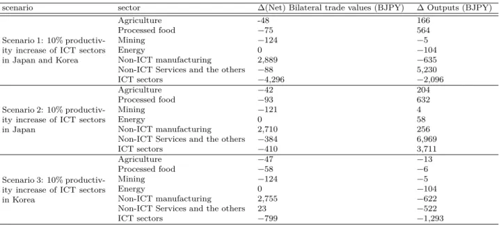
5.3. Simulations 5.3.1. Overall
We irst calculate the equilibrium price when productivity increases in the ICT sectors of Japan and Korea. For this, we use the 2000–2005 linked input–output tables of Japan and Korea. Since linked input–output tables do not provide price indexes for the primary inputs, i.e., labor and capital, we aggregate them as a single input in this paper. To address this, we adopt the quality-adjusted price indexes of labor and capital which are compiled by JIP (2015) for Japan and by KIP (2015) for Korea, for the corresponding periods to inlate the value-added observed in normal values. To construct a bilateral general equilibrium model, we use the UN Comtrade database. Domestic and trade models are integrated into this bilateral model. First, we look at what happens when the productivity of every ICT sector is increased by 10% exogenously in Japan and Korea. Using the bilateral general equilibrium model, we summarize the total efects in Table 5. We explain changes in inal demand, and in the export and import of the two countries, in three kinds of scenarios. The irst indicates that productivity improved in both countries. The second case shows that productivity increased only in Japan, while the last shows an increment only in Korea. Notice that BJPY stands for billion Japanese yen and BKRW for billion Korean won. The increase in the gross domestic product (∆GDP) from both countries’ ICT improvement is
4,343 BJPY for Japan and 77,284 BKRW for Korea. The net beneit (in terms of gain in inal demand∆y) is 8,582 BJPY for Japan (about 1.70% of the current GDP) and 54,303 BKRW
for Korea (about 6.49% of the current GDP). When only one country’s ICT productivity grows, GDP and inal demand may increase. Japan gets additional 8,292 BJPY of GDP and
9,792 BJPY of inal demand because of Japan’s ICT betterment. Meanwhile, Korea gains 40,090 BKRW of GDP and 35,042 BKRW of inal demand through Korea’s ICT productivity growth. Meanwhile, the partner’s ICT development has diferent efects. Japan’s improved ICT raises Korea’s GDP (11,452 BKRW) and inal demand (5,117 BKRW), since Korea has huge imports from Japan (53,842 BKRW). Productivity growth knocks the price down. Thus, Korea imports more of the relatively cheaper Japanese goods. However, Korea’s ICT productivity enhancement curtails Japan’s GDP (−1,142 BJPY) and inal demand (−232 BJPY). The changes in bilateral trades, i.e., exports and imports between the two countries, show positive signs in Table 5. Exports from Korea to Japan (74,856 BKRW) are greater than imports from Japan (58,667 BKRW) in the irst simulation, when ICT improves in both countries. Thus, Korea has a positive net export (16,189 BKRW). On the other hand, Japan shows negative net exports (−1,742 BJPY). However, if ICT productivity of only one side is enhanced, Korea’s exports decline sharply. Net exports of Korea in scenario 2 record −15,425 BKRW and −16,299 BKRW in scenario 3. Korea’s bilateral imports shows equivalent amounts in the three scenarios, as seen in Table 5. In other words, Korea’s economy depends deeply on Japan. Meanwhile, Japan’s bilateral imports in the second and third scenarios are less than half of those in the irst scenario. Japan responds lexibly to price changes in bilateral trade.
5.3.2. Sectoral price changes
Basically, when there is a 10% productivity improvement in one sector, prices fall by 10%. However, the intersectoral propagation of that price change will difer depending on the elasticity of factor substitution among the interacting sectors. All ICT sectors show more than 9% price reductions in Figure 8 for Japan and Figure 9 for Korea. In these igures, most of the ICT sectors show a greater than 10% price reduction.
The top six ICT sectors in Figure 8 are j = 364 (advertising services, 14.66%), j =
374 (movie theaters, 13.91%), j = 229 (radio and television sets, 13.41%), j = 234
(per-sonal computers, 12.57%),j = 236 (electronic computing equipment (accessory equipment),
12.43%), and j =327 (private broadcasting 12.14%) for Japan. Meanwhile,j = 315
(adver-tising services, 18.72%),j = 227 (television, 15.48%),j = 231 (wireless telecommunication
and broadcasting apparatuses, 14.75%),j = 301 (broadcasting, 14.20%),j = 232 (computer
and peripheral equipment, 13.69%), andj= 229 (other audio and visual equipment, 13.55%)
rank high in the two countries. It is obvious that the advertising and broadcasting industries have huge interaction in the economy. Meanwhile, computer equipment, the representative ICT indstry, ranked fourth and ifth in Japan and ifth in Korea. Moreover, not only ICT industries, but also non-ICT industries showed lower prices in response to ICT innovation, as seen in Figures 8 and 9. For examples,j =128 (cosmetics, toiletries, and dentifrices, 3.14%), j =219 (applied electronic equipment, 3.09%), j =259 (cameras, 2.90%), j =264 (medical
instruments, 2.03%), j =220 (electrical measuring instruments, 2.02%) and j =127 (soap,
synthetic detergents, and surface active agents, 1.89%) are the top six non-ICT industries for Japan, as seen in Figure 8, whereas j =238 (regulators and measuring and analytical
instruments, 3.04%),j =348 (oice supplies, 2.54%),j =235 (household laundry equipment,
2.40%),j =236 (other household electrical appliances, 2.38%), j =280 (electric power plant
construction, 2.32%), andj =237 (medical instruments and supplies, 2.13%) are the top six
for Korea, as seen in Figure 9. Thus, ICT innovation induces price reductions for itself and other industries. To take a concrete example, the two biggest inputs of j =128 (cosmetics,
toiletries, and dentifrices) industry of Japan are ICT industries such asj = 364 (advertising
services) andj = 349 (research and development (intra-enterprise)). There is one more point
we should consider. Figures 8 and 9 explain that Korea saw greater price reductions than Japan. The price cut in the ICT industry of Japan is 10.92%, on average, whereas in Korea it is 12.29%. Figures 10) and 13) show that price changes were only inluenced by domestic ICT improvement. The ICT industries’ average was 10.52% for Japan and 11.96% for Korea. The price reduction caused by only the partner country’s ICT uplift was 0.14% for Japan and 0.29% for Korea, as seen in Figures 12 and 11. In Figure 12, ICT industries such asj =
229 (radio and television sets, 1.32%), j = 234 (personal computers, 0.72%), j = 236
(elec-tronic computing equipment (accessory equipment), 0.61%), and j = 231 (cellular phones,
0.60%) are ranked high. Similarly, high ranked sectors for Korea are ICT industries such asj = 221 (semiconductor devices, 1.13%), j = 228 (household electrical audio equipment,
0.89%),j = 227 (television, 0.71%), j = 231 (wireless telecommunication and broadcasting
apparatuses, 0.70%), andj = 232 (computer and peripheral equipment, 0.67%) in Figure 11.
Ultimately, domestic ICT growth inluences the partner country’s price of ICT industries. Furthermore, Korea sufers a bigger downturn than Japan, as it is strongly afected by the partner’s economic climate.
5.3.3. Sectoral changes of outputs and bilateral trade values
To observe industrial changes speciically, we classify sectors into seven categories, in-cluding ICT industries. Here non-ICT industries are aggregated into six sectors such as
agriculture, processed food, mining, energy, non-ICT manufacturing, non-ICT services, and the others. The changes of total bilateral trade values by the three scenarios are mentioned in 5.3.1. Tables 6 and 7 demonstrate changes of (domestic) outputs and bilateral trade val-ues (net) of eight groups between Japan and Korea. Overall, Table 7 shows a larger number of positive values than Table 6. It suggests Korea gains more than Japan in terms of output. In 5.3.2, we found that chain reactions to price changes in Korea are more sensitive than in Japan. If the price of intermediate inputs drops because of any exogenous ICT productivity improvement, Korea beneits as it is more sensitive to price changes of intermediate inputs. Thus, Korea produces more with cheaper intermediate inputs. In Korea, all scenarios show an increase in output, whereas Japan has negative values under scenarios 1 and 3. This means that if there is no ICT innovation in Japan but only betterment in Korea, the output of Japan shrinks. In other words, Japan’s domestic intermediate inputs are substituted for imported goods from Korea since they become cheap. Simultaneously, net bilateral trade values of the ICT industries of Japan show negative values for all cases. On the other hand, Korea has negative net trade values for non-ICT manufacturing for all scenarios (and ad-ditional negative net trade values for non-ICT services and the others for scenarios 1 and 3), since Japan’s non-ICT goods become cheaper because of an improvement in ICT. Thus, Korea imports more non-ICT goods from Japan. This then leads to negative values in net bilateral trade values of Korea’s non-ICT industries.
6. Concluding Remarks
Table 1: ICT sectors in Japan
id sector ICT sectors
Communication 284 Telecommunication facilities construction 323 Fixed telecommunication
324 Mobile telecommunication
325 Other services relating to communication Broadcasting 326 Public broadcasting
327 Private broadcasting 328 Cable broadcasting Information services 329 Information services
330 Internet based services
Information production 331 Image information production and distribution industry 332 Newspaper
333 Publication
334 News syndicates and private detective agencies ICT-related sectors
Manufacturing 103 Printing, plate making and book binding 175 Electric wires and cables
176 Optical iber cables 210 Copy machine 211 Other oice machines
227 Video recording and playback equipment 228 Electric audio equipment
229 Radio and television sets 230 Wired communication equipment 231 Cellular phones
232 Radio communication equipment (except cellular phones) 233 Other communication equipment
234 Personal Computers
235 Electronic computing equipment (except personal computers) 236 Electronic computing equipment (accessory equipment) 237 Semiconductor devices
238 Integrated circuits 239 Electron tubes 240 Liquid crystal element 241 Magnetic tapes and discs 242 Other electronic components
268 Audio and video records, other information recording media ICT related services 364 Advertising services
374 Movie theaters
375 Performances (except otherwise classiied), theatrical companies R & D
343 Research institutes for natural science (pubic) **
344 Research institutes for cultural and social science (public) ** 345 Research institutes for natural sciences (private, non-proit) *
346 Research institutes for cultural and social science (private, non-proit) * 347 Research institutes for natural sciences (proit-making)
348 Research institutes for cultural and social science (proit-making) 349 Research and development (intra-enterprise)
also react sensitively to ICT innovation in both countries. On average, Korea has bigger cost reductions than Japan since Korea’s price reductions are large. Third, net bilateral trade values indicate that Korea gains more than Japan. Since Korea reacts quickly to price changes, it can achieve bigger cost reductions. Thus, Korea beneits more from bilateral trade.
Table 2: ICT sectors in Korea
id sector ICT sectors
Communication 281 Communications line construction 300 Telecommunications
Broadcasting 301 Broadcasting
Information services 314 Market research and management consultancy 317 Computer softwares development and supply 318 Computer related services
Information production 334 Newspapers 335 Publishing ICT-related sectors
Manufacturing 113 Printing
114 Reproduction of recorded media 212 Motors and generators
213 Electric transformers
214 Capacitors and rectiiers, electric transmission and distribution equipment 215 Insulated wires and cables
216 Batteries
217 Electric lamps and electric lighting ixtures 218 Misc. electric equipment and supplies 219 Electron tubes
220 Digital display 221 Semiconductor devices 222 Integrated circuits
223 Electric resistors and storage batteries 224 Electric coils, transformers
225 Printed circuit boards 226 Misc. electronic components 227 Television
228 Electric household audio equipment 229 Other audio and visual equipment 230 Line telecommunication apparatuses
231 Wireless telecommunication and broadcasting apparatuses 232 Computer and peripheral equipment
233 Oice machines and devices ICT-related services 315 Advertising services
336 Library, museum and similar recreation related services (public) 337 Library, museum and similar recreation related services (other) 338 Motion picture, theatrical producers, bands, and entertainers R & D
310 Research institutes (public)
Table 3: CES Elasticities and Productivity Growths of ICT sectors (Japan 2000–2005)
id sector Elasticity TFPg Obs.
103 Printing, plate making and book binding 1.548 0.084 125 175 Electric wires and cables 1.575 *** 0.044 119 176 Optical iber cables 1.636 ** -0.361 *** 113
210 Copy machine 1.240 -0.539 *** 130
211 Other oice machines 1.136 0.528 131
227 Video recording and playback equipment 2.003 *** 0.769 *** 134 228 Electric audio equipment 1.391 * 0.397 *** 144 229 Radio and television sets 0.939 -7.175 ** 123 230 Wired communication equipment 2.198 *** -0.237 *** 148
231 Cellular phones 1.141 3.126 145
232 Radio communication equipment (except cellular phones) 1.354 -0.283 ** 147 233 Other communication equipment 0.752 -0.322 * 139
234 Personal Computers 1.448 * 0.634 124
235 Electronic computing equipment (except personal computers) 1.643 *** 0.249 124 236 Electronic computing equipment (accessory equipment) 1.887 *** 0.406 *** 130
237 Semiconductor devices 1.501 0.024 122
238 Integrated circuits 1.245 -0.824 124
239 Electron tubes 1.787 *** 0.000 114
240 Liquid crystal element 2.256 *** 1.252 ** 114
241 Magnetic tapes and discs 1.506 0.357 119
242 Other electronic components 1.692 *** -0.078 150 268 Audio and video records, other information recording media 1.530 ** -0.127 * 93 284 Telecommunication facilities construction 1.279 0.129 138 323 Fixed telecommunication 0.773 0.613 ** 101
324 Mobile telecommunication 1.899 -0.156 73
325 Other services relating to communication 2.410 *** 0.016 63
326 Public broadcasting 1.170 -0.445 * 88
327 Private broadcasting 1.082 -1.626 *** 91
328 Cable broadcasting 1.104 -1.598 *** 81
329 Information services 1.439 0.028 98
330 Internet based services
331 Image information production and distribution industry 1.660 ** -0.206 ** 117
332 Newspaper 1.508 ** 0.006 97
333 Publication 1.450 * 0.027 103
334 News syndicates and private detective agencies 1.397 * -0.052 72 343 Research institutes for natural science (pubic) ** 2.069 -0.765 *** 88 344 Research institutes for cultural and social science (public) ** 2.044 -0.923 *** 62 345 Research institutes for natural sciences (private, non-proit) * 1.393 -2.078 *** 59 346 Research institutes for cultural and social science (private, non-proit) * 1.215 -5.071 *** 47 347 Research institutes for natural sciences (proit-making) 2.114 ** -0.854 *** 91 348 Research institutes for cultural and social science (proit-making) 2.396 -0.227 ** 50 349 Research and development (intra-enterprise) 1.465 ** -0.318 *** 124
364 Advertising services 1.925 *** 0.017 101
374 Movie theaters 0.484 -0.122 74
375 Performances (except otherwise classiied), theatrical companies 1.287 0.137 106
Table 4: CES Elasticities and Productivity Growths of ICT sectors (Korea 2000–2005)
id sector Elasticity TFPg Obs.
113 Printing 1.579 *** 0.072 139
114 Reproduction of recorded media 1.977 *** 0.115 * 132 212 Motors and generators 1.747 *** 0.177 ** 157 213 Electric transformers 1.815 *** 0.079 146 214 Capacitors and rectiiers, electric transmission and distribution equipment 1.562 ** -0.013 163 215 Insulated wires and cables 1.784 *** -0.098 165
216 Batteries 1.389 0.269 147
217 Electric lamps and electric lighting ixtures 1.582 ** -0.074 156 218 Misc. electric equipment and supplies 1.492 * 0.075 151
219 Electron tubes 1.695 *** 0.382 ** 155
220 Digital display 1.095 0.708 155
221 Semiconductor devices 1.511 ** 0.359 158
222 Integrated circuits 1.190 0.343 163
223 Electric resistors and storage batteries 2.063 *** 0.576 *** 152 224 Electric coils, transformers 1.334 0.448 *** 138 225 Printed circuit boards 1.540 ** 0.347 156 226 Misc. electronic components 1.402 0.497 * 166
227 Television 1.470 0.840 ** 146
228 Electric household audio equipment 2.123 *** 0.559 *** 147 229 Other audio and visual equipment 1.596 * 0.396 * 160 230 Line telecommunication apparatuses 1.645 ** 0.111 157 231 Wireless telecommunication and broadcasting apparatuses 1.501 0.915 159 232 Computer and peripheral equipment 1.630 ** 0.605 162 233 Oice machines and devices 1.543 * 0.320 ** 150 281 Communications line construction 1.576 ** 0.002 155
300 Telecommunications 1.596 * -0.237 * 119
301 Broadcasting 0.965 -2.958 119
310 Research institutes (public) 1.578 ** -0.086 178 311 Research institutes (private, non-proit, commercial) 1.523 ** 0.527 *** 148 312 Research and experiment in enterprise 1.390 ** -0.540 *** 221 314 Market research and management consultancy 1.324 0.228 91
315 Advertising services 1.141 3.545 *** 121
317 Computer softwares development and supply 1.293 0.194 111 318 Computer related services 1.322 0.999 *** 107
334 Newspapers 1.878 *** -0.056 114
335 Publishing 1.494 ** 0.131 120
Table 5: Prospective analysis of productivity improvement in ICT sectors between Japan and Korea
Japan Korea BJPY (BKRW) BKRW (BJPY) Current Gross domestic product (GDP) 505,269 851,982
Scenario 1: 10% productivity increase of ICT sectors in Japan and Korea
∆GDP 4,343 40,362 77,284 8,316
∆Final demand∆y 8,582 79,759 54,303 5,843 ∆Export to partner∆ep 6,313 58,667 74,856 8,054
∆Import from partner∆mp 8,054 74,856 58,667 6,313
∆ep-∆mp -1,742 16,189
Scenario 2: 10% productivity increase of ICT sectors in Japan
∆GDP 8,292 77,065 11,452 1,232
∆Final demand∆y 9,792 91,007 5,117 551 ∆Export to partner∆ep 5,686 52,842 37,417 4,026
∆Import from partner∆mp 4,026 37,417 52,842 5,686
∆ep-∆mp 1,660 -15,425
Scenario 3: 10% productivity increase of ICT sectors in Korea
∆GDP -1,142 -10,618 40,090 4,314 ∆Final demand∆y -232 -2,160 35,042 3,771 ∆Export to partner∆ep 5,593 51,981 35,681 3,839
∆Import from partner∆mp 3,839 35,681 51,981 5,593
∆ep-∆mp 1,754 -16,299
Table 6: Changes of Sectoral Outputs and Bilateral Trade Values (Japan)
scenario sector ∆(Net) Bilateral trade values (BJPY) ∆Outputs (BJPY)
Scenario 1: 10% productiv-ity increase of ICT sectors in Japan and Korea
Agriculture -48 166
Processed food −75 564
Mining −124 −5
Energy 0 −104
Non-ICT manufacturing 2,889 −635 Non-ICT Services and the others −88 5,230
ICT sectors −4,296 −2,096
Scenario 2: 10% productiv-ity increase of ICT sectors in Japan
Agriculture −42 204
Processed food −93 632
Mining −121 4
Energy 0 58
Non-ICT manufacturing 2,710 256 Non-ICT Services and the others −384 6,969
ICT sectors −410 3,711
Scenario 3: 10% productiv-ity increase of ICT sectors in Korea
Agriculture −47 −13
Processed food −58 −6
Mining −124 −5
Energy 0 −104
Non-ICT manufacturing 2,755 −622 Non-ICT Services and the others 23 −522
ICT sectors −799 −1,293
Table 7: Changes of Sectoral Outputs and Bilateral Trade Values (Korea)
scenario sector ∆(Net) Bilateral trade values (BKRW) ∆Outputs (BKRW)
Scenario 1: 10% productiv-ity increase of ICT sectors in Japan and Korea
Agriculture 334 2,507
Processed food 828 4,465
Mining 1,472 211
Energy 0 1,508
Non-ICT manufacturing −20,123 39,039 Non-ICT Services and the others −469 56,724
ICT sectors 34,147 82,844
Scenario 2: 10% productiv-ity increase of ICT sectors in Japan
Agriculture 340 354
Processed food 940 795
Mining 1,417 61
Energy 0 449
Non-ICT manufacturing −22,419 13,984 Non-ICT Services and the others 160 9,260
ICT sectors 4,138 14,059
Scenario 3: 10% productiv-ity increase of ICT sectors in Korea
Agriculture 324 1,437
Processed food 680 2,506
Mining 1,479 128
Energy 0 519
Non-ICT manufacturing −24,085 12,536 Non-ICT Services and the others −481 29,375
ICT sectors 5,784 29,150
0
5
10
15
price cut (%)
0 100 200 300 400
sector
0
5
10
15
20
price cut (%)
0 100 200 300 400
id
Figure 9: Sectoral distribution of price cut of Korea (10% of ICT productivity increments in Japan and Korea)
0
5
10
15
price cut (%)
0 100 200 300 400
sector
Figure 10: Sectoral distribution of price cut of Japan (10% of ICT productivity increments only in Japan)
0
.5
1
price cut (%)
0 100 200 300 400
id
0
.5
1
1.5
price cut (%)
0 100 200 300 400
sector
Figure 12: Sectoral distribution of price cut of Japan (10% of ICT productivity increments only in Korea)
0
5
10
15
20
price cut (%)
0 100 200 300 400
id
Figure 13: Sectoral distribution of price cut of Korea (10% of ICT productivity increments only in Korea)
References
BOK, 2009. 1995, 2000, 2005 Linked Input-Output Tables [in Korean]. Economic Statistics System. Bank of Korea. URL:http://ecos.bok.or.kr.
Comtrade, 2017. UN Comtrade Database. URL:https://comtrade.un.org.
Farhadi, M., Ismail, R., Fooladi, M., 2012. Information and communication technology use and economic growth. PLoS ONE 7. doi:10.1371/journal.pone.0048903.
JIP, 2015. Japan Industrial Productivity Database. URL:
http://www.rieti.go.jp/en/database/jip.html.
Jorgenson, D.W., Motohashi, K., 2005. Information technology and the Japanese economy. Journal of the Japanese and International Economies 19, 460–481.
Ju, J., 2014. The efects of technological change on employment: The role of ICT. Korea and the World Economy 15, 289–307.
Jung, H.J., 2012. ICT Industrial structure and input-output analysis [in Korean]. Technical Report 563. Korea Information Society Development Institute.
Jung, H.J., Na, K.Y., Yoon, C.H., 2013. The role of ICT in Korea’s economic growth: Productivity changes across industries since the 1990s. Telecommunications Policy 37, 292–310.
doi:10.1016/j.telpol.2012.06.006.
Kanamori, T., Motohisa, K., 2007. Information Technology and Economic Growth: Comparison between Japan and Korea. Discussion Paper 07-E-009. Research Institute of Economy, Trade and Industry. Kecek, D., Hrustek, N.Z., Dusak, V., 2016. Analysis of multiplier efects of ICT sectors - a Croatian case.
Croatian Operational Research Review 7, 129–145. doi:10.17535/crorr.2016.0009. Kim, J., Nakano, S., Nishimura, K., 2017. Bilateral multifactor CES general equilibrium with
state-replicating Armington elasticities. Asia-Paciic Journal of Regional Science , 1–22doi:10.1007/s41685-017-0068-7.
Kim, J.E., Jung, H.J., Lee, Y.S., Yang, H.S., Kim, M.J., Song, J.K., 2016. A study on time-series method of ICT input-output tables [in Korean]. Jinhanbook.
KIP, 2015. Korea Industrial Productivity Database. URL:
https://www.kpc.or.kr/eng/Productivity/kip.asp.
Krasnosel’skiĭ, M.A., 1964. Positive Solutions of Operator Equations. Groningen, P. Noordhof.
Kwak, K., 2014. Status and future trend of value-added induction of ICT convergence in manufacturing [in Korean]. Technical Report 1672. Institute for Information & Communications Technology Promotion. Lee, S.Y.T., Gholami, R., Tong, T.Y., 2005. Time series analysis in the assessment of ICT impact at the
aggregate level - lessons and implications for the new economy. Information & Management 42, 1009–1022.
Mattioli, E., Lamonica, G.R., 2013. The ICT role in the world economy: an input-output analysis. Journal of World Economic Research 2, 20–25. doi:10.11648/j.jwer.20130202.11.
MIAC, 2011. 1995–2000–2005 Linked Input–Output Tables [in Japanese]. Technical Report. Ministry of Internal Afairs and Communications. URL:http://www.soumu.go.jp/main_content/000291877.pdf. MIAC, 2017. A report on ICT input-output tables [in Japanese]. Technical Report. Ministry of Internal
OECD, 2011. Guide to measuring the information society. Technical Report. OECD publishing. doi:10.1787/10.1787/9789264113541-en.
OECD, 2017. Digital Economy Outlook 2017. Technical Report. OECD publishing. doi:10.1787/9789264276284-en.
Vu, K.M., 2013. Information and communication technology (ICT) and singapore’s economic growth. Information Economics and Policy 25, 284–300. doi:10.1016/j.infoecopol.2013.08.002. Xing, W., Ye, X., Kui, L., 2011. Measuring convergence of China’s ICT industry: An input-output
analysis. Telecommunications Policy 35, 301–313. doi:10.1016/j.telpol.2011.02.003. Zuhdi, U., Mori, S., Kamegai, K., 2012. Analyzing the role of ICT sector to the national economic
structural changes by decomposition analysis: The case of Indonesia and Japan. Social and Behavioral Sciences 65, 749–754.