Real-time and Efficient Rendering of Deformable Bodies

(1)

Deformable Bodies

著者 LAZUNIN Vladimir page range 1‑83

year 2016‑09‑15

学位授与番号 32675甲第609号学位授与年月日 2016‑09‑15

学位名博士(理学)

学位授与機関法政大学 (Hosei University)

URL http://doi.org/10.15002/00013343

(2)

Real–time and Efficient Rendering of Deformable Bodies

Vladimir Lazunin

(3)

List of Figures

1.1 Level of details and corresponding deformability: only two triangles are enough to represent a flat sheet of rigid material (left), that cannot be deformed realistically without a sufficient increase in polygon count (right). . . 2

2.1 Sunflowers (1 billion triangles) and Boeing 777 (370 million triangles) from the works of Wald et al. [1], [2]. Scenes of such complexity are much easier to render with ray tracing than with rasterizing. . . 18 2.2 Scheme of simple, non–recursive ray tracing. Two rays are shown: R1hitting andR2missing the

scene object (the circle). Solid line S represents the screen. Using cosine law, the screen point P1is going to have the same (R, G, B) color as the object material, multiplied by cosα, whereα is the angle between −R1 and the object’s surface normal at the hit point. . . 19 2.3 Simple non–recursive ray tracing of a green plane and three white spheres. Orange is used as the

background color, and cosine law is used for shading. . . 20 2.4 Shadow rays in recursive ray tracing. Primary rays are cast from the camera, spawning secondary

shadow rays, originating at their points of intersection with the ground plane and directed towards the light source L. Where these shadow rays are blocked by scene objects and unable to reach the light source, a shadow is created. . . 20

(6)

2.5 Reflection and refraction rays in recursive ray tracing. Primary ray Rprimary spawns two secondary rays: a reflection ray Rref l and a refraction rayRref r. Possibly intersecting other scene objects, these ray bring back some additional color information, which is then blended according to the selected coloring scheme, creating reflection and refraction. . . 21 2.6 Recursive ray tracing of a semi–transparent colorless bell and two planes with procedural check-

ered textures. Reflection, refraction and light attenuation can be seen on the bell, and a shadow effect — on the floor underneath it. . . 22

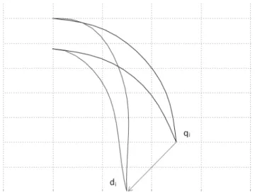
3.1 An example of a creature, with a deformation vector assigned at the bell margin. qi designate the initial position of the bell margin point (rest shape), di – the fully deformed position of the same bell margin point. . . 37 3.2 Animation sequence of a single contraction–expansion cycle of a jellyfish. The contraction phase is

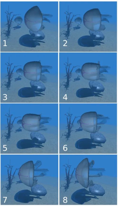
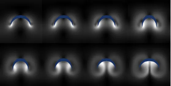
shown with frames 1–4, the expansion phase — with frames 5–8. Floating tentacles are animated according to the water velocity field. Small additional deformations are applied to the bell for a more realistic look. . . 42 3.3 Formation of a vortex in 2D during one full expansion–contraction step (the expansion is shown

in the top row, the contraction – in the bottom row, left to right). . . 43

4.1 While garment models can be pre–made to fit a given human figure one by one, they cannot be pre–made to also fit each other in all possible combinations. Left to right: pants fitting correctly;

dress fitting correctly; interference between dress and pants; desired result. . . 47 4.2 Basic idea: rays (dashed arrows), the higher layerM²(solid line) and the lower layerM¹(dashed

line). Problematic area (a) with M¹ showing through M²; same area after fixing visually by

”ignoring”M¹(b) and geometrically by deformingM¹ to be positioned correctly (c) . . . 55 4.3 A simple case: interference and z-fighting of two sheets of deformable cloth and rigid floor, collided

together (left) resolved visually (right) . . . 55

(7)

4.4 A na¨ıve implementation used on two garments: a white dress (solid line in 2D view) worn over a red shirt (dashed line in 2D). All cloth interferences and incorrect positioning are resolved, except for the left and right sides, where the red shirt is still incorrectly shown. This happens because rays are missing one of the garments entirely at the silhouette edges (a). The proposed solution is to trace a secondary ”probe ray” in the direction opposite to the surface normal (b). . . 56 4.5 The arm ”disappearing” if seen from the left, because probe rays find a higher layer object (red

shirt). The proposed solution is to limit the probe ray search distance to a certain valuel, roughly equal to the body part ”radius”. . . 57 4.6 Folds and drapes of a 3D garment, making geometrical surface normal change its direction to be

parallel or opposite of the surface normal ”in general”. In such cases, using geometric surface normals to direct the probe rays still causes them to miss garments (a). The proposed solution is to assign additional vectors (”global normals”) to guide the probe rays (b). . . 58 4.7 Body parts segmentation, representing the ray tracing hierarchy: corresponding parts are traced

only against each other. The skirt is traced against both thighs and the torso. . . 59 4.8 Boundary and non–boundary edges of a triangular mesh surface (shown in grey). Edges with

only one adjacent triangle (EA,ABandBF on the picture) are considered boundary edges, and points adjacent to them (E,A,B andF on the picture) — boundary points. . . 60 4.9 Recursively gathering topological neighbors of a triangle: the original triangle (red), the first level

neighbors (green) and the second level neighbors (blue). . . 61 4.10 Camera rays (dashed arrows) and probe rays (solid arrows) and a problem that appears near a

boundary edge of the green pants due to the green and red surfaces being too far apart (a); visual gap (b) and over–stretched edge (c) near the boundary. Solid line represents the outer layer of clothing (M²), dashed line — the inner layer of clothing (M¹). . . 61 4.11 Performance of layered ray tracing on two different GPUs: computation time does not increase

proportionally to the number of triangles. . . 65

(8)

4.12 A test run: a human dressed in a jumpsuit, pants and two different shirts, 249644 triangles total.

Front (a) and back (b) views of the same configuration are shown side by side in their original (left) and resolved (right) states. . . 66 4.13 A test run: a human dressed in pants, shirt and two dresses, 121064 triangles total. Front (a)

and side (b) views of the same configuration are shown side by side in their original (left) and resolved (right) states. . . 66 4.14 Cloth interference (left), polygons showing through in a concave area after all vertices were

geometrically corrected (middle) and the same problem corrected visually (right). . . 67 4.15 A test run: two polygonal sheets of cloth falling onto several collision primitives. Z–fighting,

cloth–cloth and cloth–body interference due to imprecise physical simulation (left); same scenes after visual correction (right). It can be seen on the right, that some folds of the underlying red sheet were ”flattened” by this correction, as well as sharp edges of the green cube were ”smoothed”. 68 4.16 Performance chart for the test data acquired during the tests simulations of 1 to 4 sheets of

cloth interacting with several colliding primitives. Dashed line represents simple ray tracing, solid line — layered ray tracing. Black colored lines represent average, red colored lines — worst case performance (both values measured over 500 frames of simulation). Note that for the same triangle count less time is required if all the cloth triangles belong to a single layer, than when they are divided between 2, 3 or 4 layers. . . 70

(9)

List of Tables

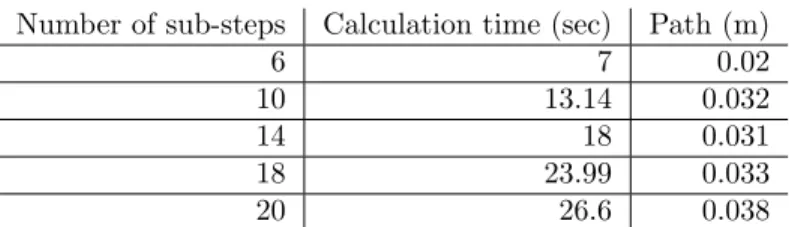
3.1 Performance results of Aurelia aurita jellyfish simulation, showing how the number of simulation substeps (temporal resolution) affects the calculation time and the distance, travelled by the jellyfish. . . 41

4.1 Performance test results for simple ray tracing and our layered ray tracing of the same scenes consisting of several rigid primitives and from 1 up to 4 sheets of cloth of different resolution. 500 frames were generated for each simulation, average and worst–case performance data is provided. 69

(10)

Acknowledgments

I would like to thank my advisor professor V. Savchenko for guiding me in my research. I also want to express my gratitude to professors N. Koike, T. Koike, S. Fujita and T. Wakahara for their invaluable and timely feedback regarding this thesis.

(11)

Chapter 1

Overview of existing methods of deformable body simulation and 3D visualization

1.1 General Introduction

Deformable bodies form a wide category of objects important for numerical computation in general, and computer graphics, in particular. In fact, most, if not all real life objects can be qualified as ”deformable”

– however, when it comes to computational models, the deformability aspect is not as widely used. The reasons are many: for some cases elasticity is not big enough to be important, and therefore using only rigid body dynamics is justified. In many cases, however, elasticity is essential, but still cannot be used due to forbiddingly high computational cost. Some real life objects are treated differently, depending on a particular application: for example, a car may be treated as a rigid body when simulating physical interactions for a computer game, but as a deformable body for a numerical crash simulation. The complexity of underlying physical simulation methods may vary accordingly: for a game, simple – and not too physically accurate – bouncing calculated with rigid body dynamics would be enough, while very accurate deformations are calculated for a crash test using, for example, the finite element method (FEM). Between such extreme cases lies the area where only some aspect of the deformable behavior matter, or no high precision is required as

(12)

long as the visualization result looks convincing. This includes movies, virtual reality (VR) and augmented reality applications, video games and so on. Good examples are clothing and hair simulation: the numerical models vary greatly, from very simple ones with real–time performance, used in games and VR applications, to very complicated, which may require hours of computation to provide realistic results to be used in a movie scene. In games, for example, human characters design is still very much restricted in the ways that allow treating clothing and hair as rigid, inseparable parts of the body, because more realistic cloth simulation would require more computations as well as higher resolution models (see Fig. 1.1 for a simple example).

Figure 1.1: Level of details and corresponding deformability: only two triangles are enough to represent a flat sheet of rigid material (left), that cannot be deformed realistically without a sufficient increase in polygon count (right).

This chapter provides a survey of the methods that are used for deformable body simulation and, in more general terms, deformable body representation in computer graphics domain, as well as a survey and general descriptions of visualization methods used in computer graphics. Problem statements and the goals of the thesis are formulated in this chapter. Surveys of more specific techniques, tied more closely to the problems solved in the thesis, are provided in their respective chapters.

1.2 General classification of methods used for deformations simulation

To summarize the historical review given above, here is a broad categorization of methods used for simulating deformable bodies in computer graphics. More technical details, as well as further references regarding each category can be found, for example, in a technical report of Gibson and Mirtich [3].

There are more than one way to classify the methods, but, perhaps, the most important divisions are

(13)

implicit/parametric anddiscrete/continuous. In implicit methods the deformations are not applied directly to the body of interest, but rather the space around it, or a primitive the body is embedded into, changes the shape, implicitly causing the body to deform accordingly. In parametric methods, on the other hand, the deformations are introduced directly into the equations of the deformable body as parameters (hence the name ”parametric”). In discrete methods, the body shape is approximated by a discrete set of elements, and all deformations are applied only to those elements. In continuous methods, the body is treated as a monolithic entity, with its properties continuously changing throughout the body. It is important to note, however, that this distinction between discrete and continuous methods applies only to the representation of the body itself — it has nothing to do with the methods used to solve underlying equations: numerical methods will be discrete for both cases.

Curves, Splines and patches

Catenary curves, introduced by Leibniz, Huygens and Bernoulli in 17th century to describe shapes of a hang- ing chain, are used in some cloth simulations. Obviously, this approach is quite limited, but computationally efficient. The equation of a catenary in Cartesian coordinates is

y=acosh(x a) =a

2(e^x/a+e^−x/a) (1.1)

B´ezier curves and surfaces, B–splines, rational B–splines, non–uniform rational B–splines and many other methods of specifying curves and surfaces with a relatively small number of control points are widely used in computer–aided design (CAD) to model deformable objects. They allow a high degree of control and are computationally efficient to deform (but not to visualize, for that purpose they are usually split into sets of flat triangles). However, they are not very suitable for automatic deformations which occur, for example, in response to pressure or collision, and may require a lot of manual labour to adjust the control points to achieve desired shape changes.

(14)

Free–form deformation

Free–form deformation (FFD) deforms an object by deforming the space in which the object lies. It is a very general technique and can be applied to many graphical representations, such as polygons, splines, parametric patches and implicit surfaces. In general, it can be expressed as a space mappingf :R³→R³. Because the possible regions and types of deformations are limited, the object is usually embedded into a cubical or cylindrical lattice of grid points, forming a set of three–dimensional cells {Ui}. The free–form deformation thus becomes a collection of mappings in the formfi:Ui →R³.

Mass–spring systems

Mass–spring systems, as the name suggests, is a physically–based technique of approximating a deformable object by a set of mass particle, interconnected by springs, usually in a lattice pattern. The spring forces may be linear, according to the Hooke’s law, or non–linear, to model inelastic tissues. During the simulation process, the sum of forces is calculated for every mass point. It includes forces exerted by the springs connected to the point, as well as the external forces, if applicable. The point is, then, moved according to Newton’s Second Law.

With mass–spring system, real–time performance can be achieved with today’s commodity computers.

They are easy to construct and animate, and are widely used in deformable body simulation, such as facial and cloth simulation and so on. It is, however, difficult to model some of the aspects of soft tissues, such as incompressibility. This problem can be solved by introducing additional forces to preserve the volume, or even simply additional springs — obviously, however, that increases the computational cost. Mass–spring system can also exhibit poor stability for nearly rigid bodies.

Finite element method

While the finite element method (FEM) is a numerical technique for finding approximate solutions to boundary value problems for partial differential equations in general, and as such can be used in modeling of wide

(15)

variety of physical phenomena, in the context of this work we are going to discuss it with regard to deformable body simulations only. Unlike mass–spring models, which are discrete by nature, more accurate physical techniques model deformable object as a continuum, with mass and energy existing not only in the nodes, but distributed throughout the object. The models are derived from equations of continuum mechanics, however, it is important to note that the numerical methods used to solve the equations are still discrete.

Potential energy of a deformable body is given by:

Π = Λ−W, (1.2)

where Λ is the total strain energy of the deformable objects, and W is the work done by external forces on the deformable object. The object reaches equilibrium when its potential energy is minimal. To determine the equilibrium shape of the body, both Λ and W are expressed in terms of the object deformation. The potential energy reaches its minimum when the derivative of Π with respect to the material displacement is zero. Because it is not always possible to find an analytic solution, FEM divide the object into a set of elements (such as triangles and quadrangles in 2D, tetrahedrons and hexahedrons in 3D) and approximate the equilibrium equation over each element. FEM is much more physically realistic than mass–spring systems, but it also has much higher computational requirements. Therefore, it is mostly used in applications where precision is valuable and real–time performance is not required, such as mechanical engineering, an iconic application being a crash test.

Approximate continuum models

These are physically–motivated models, where some laws of physics are used to achieve desired effects, but usually strict adherence to the laws of physics is not the goal. Active contour models, or ”snakes” are used to find contours of static or moving objects. Snakes are deformable bodies that respond to external forces (for example, image intensity to find contours) and resist to stretching and bending, thus finding a compromise between, for example, points with high gradient on an image and a curve with minimal bending energy —

(16)

this effectively attracts the snake to image edges, while keeping its shape smooth. There are other continuum models for deformable curves, surfaces and solids, used in animation applications.

Low degree of freedom models

Discretization of a physically–based model into a large number of nodes characterized by their masses, positions and velocities leads to systems with many degrees of freedom. Such general systems support a wide variety of deformations, but they are slow to simulate. Low degree of freedom models limit the deformable object to fewer degrees of freedom, sacrificing generality for speed. This is achieved, for example, by separating geometry and dynamics, as in [4], or using constraints to connect globally deformed non–rigid pieces into complex models, as in [5]. There are also techniques to add physical behavior to parametric surface patches by minimizing an energy functional defined on the surface. The surface is restricted to a class by control point locations and weights, and the methods of constrained optimization are used to find a state vector that minimizes the energy functional while satisfying the constraints.

1.3 General overview of 3D rendering techniques

3D rendering is, essentially, the process of creating a 2D image from a 3D scene. The earliest examples of 3D rendering used simple wireframe representation of objects with different techniques for hidden lines removal and without any shading. As the computational power grew, shading became possible to generate more realistic images (although wireframe–based rendering is still in use today). In 1970 Bouknight developed LINESCAN algorithm [6] for producing computer generated half–tone presentations of three–dimensional polygonal surface structures. A technique calledflat shadingshades each polygon based on its surface normal and the direction of the light source. More advanced smooth shading techniques were introduced by Gouraud in 1971 [7] and Phong in 1975 [8] — in contrast to flat shading, with these techniques the color changed from pixel to pixel, not from polygon to polygon. Texture mapping for 3D graphics was first used by Catmull [9]. Blinn [10] introduced a technique now calledbump mapping, which allowed to simulate small dents and

(17)

wrinkles on the surface.

To add more realistic lighting to 3D scenes, different numerical approximation to therendering equation are used. The rendering equation, introduced independently in works of Kajiya [11] and Immel [12] is:

Lo(x, ωo, λ, t) = Le(x, ωo, λ, t) + Z

Ω

fr(x, ωi, ωo, λ, t)Li(x, ωi, λ, t) (ωi · n) dωi (1.3)

where

• λis a particular wavelength of light

• t is time

• xis the location in space

• nis the surface normal at that location

• ωois the direction of the outgoing light

• ω_i is the negative direction of the incoming light

• L_o(x, ω_o, λ, t) is the total spectral radiance of wavelengthλ directed outward along direction ω_o at timet, from a particular positionx

• Le(x, ωo, λ, t) is emitted spectral radiance

• Ω is the unit hemisphere centered around ncontaining all possible values forωi

• R

Ω. . . dωi is an integral over Ω

• f_r(x, ω_i, ω_o, λ, t) is the bidirectional reflectance distribution function, the proportion of light reflected from ω_i toω_oat position x, timet, and at wavelengthλ

• Li(x, ωi, λ, t) is spectral radiance of wavelengthλcoming inward towardxfrom directionωiat timet

(18)

• ωi·nis the weakening factor of inward irradiance due to incident angle, as the light flux is smeared across a surface whose area is larger than the projected area perpendicular to the ray, often written as cosθi.

Solving this equation is the primary challenge in realistic rendering. One of the approaches is based on finite element method and called radiosity algorithm. Developed in 1950 for modeling of heat transfer, it was adapted to 3D rendering in the work of Goral et al. [13] Their method modeled the interaction of light between diffusely reflecting surfaces and allowed to model effects such as diffuse light sources, soft shadows and ”color–bleeding” effect caused by diffuse reflections. Another approach, based on Monte Carlo methods, has led to methods such as photon mapping, path tracing and Metropolis light transfer.

Although very general, the equation does not model the whole range of lighting effects — for example, phenomena such as light transmission or subsurface scattering are not taken into account. The rendering equation was further generalized into a volume rendering equation by Kajiya [14].

Two major techniques used today to convert an illuminated, shaded and textured 3D scene into its final 2D representation on the screen surface areray tracing andpolygon rasterizing. Polygon rasterization is based on projecting vertices of the polygons the scene is made of onto the screen surface, then using interpolated values for lighting, shadowing, textures and so on inside the projected polygons. Rasterization sacrifices visual realism for speed, and is typically used for interactive applications, such as games. Usually there is specialized hardware for rasterization inside today’sgraphic processor units (GPU), available through standardized interfaces, such as OpenGL and DirectX.

Ray tracing, or calculation of paths and intersections of rays, waves or particles with different media is used in several fields of science and engineering, for example, to calculate sound, radio, seismic and light waves propagation and optical system design. It is also a computer visualization technique based on similar principles of light propagation, and further in this work we use the term ray tracing only in relation to visualization. Ray tracing is mainly used for more realistically looking, but not real–time visualization. It is based on an idea of rays cast from the eye, through the screen plane and onto the scene. Speaking in terms

(19)

of today’s digital displays, basically, one ray is cast per screen pixel, from the eye and towards that pixel, and then further into the scene. The pixel is then colored according to the object the ray intersects, as well as any additional information that may be present (light sources, shadowing, textures and so on). Obviously, that is the opposite of what happens in nature, where light travels from the light sources, gets reflected from the objects and then part of it comes into the eye, but in many cases such ”change of direction” is justified, because the light that does not enter the eye is of no interest.

Ray tracing for 3D visualization was introduced in 1968 by Appel [15]. His goal was to improve line–based printouts produced by digital plotters by adding shadowing. The next big advancement of that technique was done in 1979 by Whitted [16]. He introduced recursive ray tracing, where each ray hitting an object can cast several new rays of three types: reflection, refraction and shadow rays. A reflection ray travels in the mirror–reflection direction, a refraction ray’s direction is determined by its parent’s direction and the refractive properties of the transparent materials. Shadow rays are traced toward each light and determine the illumination intensity. The contribution of each secondary ray is then taken into account when calculating the resulting color of the screen pixel. Reflected and refracted rays, when hitting other objects, may produce their own reflection, refraction and shadow rays, and so on, in a recursive manner. This algorithm is widely used in ray tracing today, often being called ”whitted–style ray tracing”. In early works, term ”ray casting”

was also used interchangeably with ”ray tracing”, but recently ”ray casting” is mostly used to call simple forms of ray tracing, that do not recursively trace secondary rays.

Although it is more economical to trace rays from the eye (and tremendously wasteful, if at all possible, to trace every ray from every light source), not every phenomenon can be represented with this approach.

For example,caustics¹cannot be rendered that way. Therefore, algorithms that shoot rays from light sources as well as from the eye were also developed. These algorithms are sometimes called backwards ray tracing, although ray directions are not ”backwards”. Terms eye–based ray tracing and light–based ray tracing are also used.

Photon mapping, a two–pass global illumination algorithm, was introduced by Jensen [17]. At the 1st

1Bright patterns of light caused by focusing from wide surfaces onto a narrow area

(20)

pass, light packets called photons are cast from the light sources, and their intersections with the scene objects are stored inphoton maps. At the 2nd pass, the rendering equation is solved to calculate the surface radiance. With this approach, caustics, diffuse interreflection and subsurface scattering can be added to the rendered scene. Although originally designed to work with ray tracers, photon mapping can be extended to work with polygon rasterizing algorithms.

1.4 Problem statement and the goal of the thesis

There are two major application domains for deformable body simulations. One is where they mainly serve artistic purposes, such as painting, sculpting and various kinds of 3D modeling. There simulation techniques are creative instruments, and although both physically and non–physically–based techniques may be employed, in general obeying the laws of physics is not the goal. The other domain is where they are used to simulate deformation and elasticity phenomena seen in real life. The methods used to simulate such deformations are usually physically–based.

The goal of our research is to develop fast, real–time techniques for rendering practically important cases of deformable bodies used for real life phenomena simulations and today dominated by purely physically–

based methods. Although physics simulation is good for generality, in many cases (for example, multiple garment simulation) physically–based methods are too slow to achieve both satisfactory visual appearance and real–time speed at the same time.

This thesis presents a new hybrid technique based on three key parts:

1. Simplified physical simulation. We neither develop new physically–based methods nor contribute to any existing physically–based method. The key difference between our approach and most others is that, instead of making the physical simulation more sophisticated, we use simpler methods that have already been proven to be fast. For a big part of this thesis we used NVidia PhysX library, but our approach is not tied to it in any particular way, so other libraries (for example, Bullet Physics) or physically–based methods can be used as well.

(21)

2. Specialized recursive ray tracing–based visualization. While simple physical simulation is fast, by itself it certainly cannot achieve good results in most cases (especially since many of those cases would be problematic even for more sophisticated physically–based methods). A lot of problems remain unresolved by the physical simulation, in form of relatively small numerical errors, resulting in incorrect visualization. In our work we extend capabilities of recursive ray tracing to be able to detect and correct such errors in real–time. We call our method layered ray tracing.

3. Radial basis function (RBF)–based geometrical deformations. With simplified physics providing results that aremostly physically correct, and layered ray tracing correcting small (but numerous) simulation errors, there are still some cases that cannot be handled by those two techniques only. Such, relatively rare, cases are too problematic for the physically–based methods, producing simulation errors too big to be corrected by the layered ray tracing in a realistic–looking way. RBF–based geometrical deformations are employed for such cases to improve the results of the physical simulation before layered ray tracing is applied.

This thesis is organized as follows. Chapter 2 explains the techniques our work is based upon, as well as describes our general approach to the problem. RBF space mapping and recursive ray tracing, used throughout this work, are presented there. A technique for non–physically–based deformation of solid bodies is presented in Chapter 3. A case study of evolutionary optimization of a jellyfish is used in that chapter to validate the proposed technique. Chapter 4 presents a technique for multi–layered garment rendering, a practical case of a more general problem of cloth–cloth interference. Additional introductory sections are present at the beginning of chapters 3 and 4 to explain problems more specific to the techniques presented there: fluid–solid interaction and marine animals study in Chapter 3; garment modeling and textile simulation in Chapter 4.

(22)

Chapter 2

General methodology and approach to rendering deformable bodies

2.1 Introduction

In this chapter we present a set of general techniques we developed through the course of this work and used in later chapters. Our general approach is based on modification, adaptation and combination of three major techniques: physical simulation, RBF–based space mapping and recursive ray tracing.

The rest of this chapter is organized as follows: in the sections 2.2 – 2.4 we introduce physical simulation, RBF space mapping and recursive ray tracing, respectively, both in general terms and in the context of our work, comparing to other methods, if possible, and stating our contribution, where applicable. Then, in the sections 2.5 and 2.6 we discuss spatial hierarchical structures and GPU acceleration, applicable to both physical simulation and ray tracing. We give a brief summary of this chapter in section 2.7.

2.2 Physical simulation

There are several primary physical concepts to consider related to deformable body simulation: elasticity, stress andstrain. Elasticity is the property of a body which allows it to restore its original shape after the

(23)

forces which caused deformations are removed. The stress is the force applied to the body divided by the area of the surface to which it is applied. It is, essentially, same as pressure, and can be measured in the units of pressure,pascals, where one pascal is equal to one newton of the force applied over one square meter of surface. The strain is the relative deformation of a body, caused by stress, e. g. for an elastic rod of length Lchanging its length by ∆Ldue to the force pulling on the end, the strain is ∆L/L. Material’s elasticity is described by a stress–strain curve, which shows the relationship between stress and strain. Three primary characteristics related to stress and strains are:

• Young’s modulusdescribes how an object deforms along an axis when opposing forces are applied along that axis.

• Theshear modulus is an object’s tendency to deform without changing its volume and surface area.

• The bulk modulus describes how an object deforms in all directions when uniformly loaded in all directions, changing its volume.

For most materials the stress–strain relationship is linear for small deformations and can be described by Hooke’s law. If stress is higher than the elastic limit for the material, the stress–strain relationship is no longer linear, and for even higher stresses the material exhibitsplastic behavior, not restoring its original shape after the stress is removed. Because continuum mechanics equations are too computationally expensive to solve in real–time, simpler models, such as mass–spring systems are typically used for an approximation.

In addition to integrating equations of the chosen mechanical model of deformation, collision detection is crucial for realistic interaction between deformable (and rigid) bodies. While collision handling may be easy for small datasets of simple geometry, as the number of colliding objects and their complexity (for example, polygon count) grow, comprehensive methods for ensuring correct collision handling become impractical to implement. This is not just because the computation time becomes too big. Other problems include numerical errors, poor stability, slow convergence, geometrical singularities and oscillatory solutions.

Furthermore, in many cases (notably, multiple cloth simulation, which we discuss in more details in chapter

(24)

4) the system tends to enter physically incorrect states, which may require special handling (this is well illustrated by Volino and Magnenat–Thalmann [18]).

The approach we take in this work is not to develop a new physically–based method that does not have some of the aforementioned problems and limitations of existing physically–based methods, but to use alternative techniques to circumvent those problems and limitations. For this reason we tried to use third party physical engines whenever possible, instead of implementing physical simulations by ourselves. We used NVidia PhysX engine for basic cloth simulation in chapters 3 and 4: it provided simple physical behavior, sufficient for simpler applications, such as games, but not good enough for more sophisticated problems we are trying to solve. Therefore, we did not have to implement physical aspects of cloth simulation, rigid body simulation for the rest of the scene, forces such as gravity and friction, collision detection/response and so on — all that we got for free from PhysX. We then used RBF space mapping and recursive ray tracing to geometrically and visually improve those results.

2.3 RBF space mapping

A radial basis function (RBF) is a real–valued function whose value depends solely on the distance from a specified origin point, so that

φ(x, c) =φ(kx−ck), (2.1)

where c is the origin. Any functionφ, satisfying the equation 2.1 is a radial basis function. Their sums are often used to approximate other functions. The approximation has the form

y(x) =

N

X

i=1

wiφ(kx−xik), (2.2)

where the function y(x) is represented as a sum of N radial basis functions, associated with different origins x_i. The coefficients w_i, called weights, can be found through the linear least squares method. To build this kind of approximation, we don’t have to know the target function, only a set of its values at some

(25)

points. In this sense such approximation can also be regarded as a simple single–layer neural network, and used in time series prediction and control of non–linear systems.

We use these properties of RBF approximation in our work to create mapping functions, used for implicit space deformation. We consider a mapping function as a thin-plate interpolation. For an arbitrary area Ω, the thin–plate interpolation is a variational solution that defines a linear operator T when the following minimum condition is used:

Z

Ω

X

|α|=m

m!/α!(D^αf)²dΩ→min, (2.3)

wheremis a parameter of the variational function andαis a multi-index. It is equivalent to using the RBFs φ(r) =rlog(r) orr³form= 2 and 3 respectively, where ris the Euclidean distance between two points.

The volume splinef(P) having values hi at N pointsPi is the function

f(P) =

N

X

j=1

λjφ(|P−Pj|) +p(P), (2.4)

where p=ν0+ν1x+ν2y+ν3z is a degree-one polynomial. To solve for the weightsλj we have to satisfy the constraintshiby substituting the right part of Equation (2.4), which gives

hi=

N

X

j=1

λjφ(|Pi−Pj|) +p(Pi). (2.5)

λandν are the coefficients that satisfy a linear systemT x=b, where

T =





 A B^T

B D





 ,

x= [λ₁, λ₂, ..., λ_N, ν₀, ..., ν₃]^T, b= [h₁, h₂, ..., h_N,0,0, ...,0]^T

(2.6)

MatrixT consists of three blocks: a square sub–matrix A= [φ(|Pi−Pj|)] of sizeN×N, a zero sub–matrix D= 0 of size 4×4 in 3D case or 3×3 in 2D case, and a sub–matrix B=p(P_i) of size N×4 (N×3 for 2D cases). For 2D and 3D cases we callf(P) a volume spline. An important property of such interpolation

(26)

is its ”smoothness”, which means that the bending energy is minimal, as shown, for example, by Carr et al. [19]. We use this property for realistically–looking deformations, completely replacing physically–based simulation with RBF space mapping for jellyfish deformations in chapter 3, and combining it with simplified physical simulation of cloth in chapter 4.

2.4 Recursive ray tracing

General description and comparison with polygon rasterization

Rendering techniques widely used today fall in two categories: ray tracing and polygon rasterization. Ray tracing is based on simulating rays of light travelling from light sources and into the eye. It is a very general technique which can be used to accurately portray a wide range of rendering effects, such as shadows, reflection and refraction, dispersion and so on. Its usage is not limited to polygonal models, as it can be used to visualize any object for which a ray intersection point can be computed: analytical functions of all kinds in their explicit or implicit form, voxel data and so on.

Rasterization is based on projecting vertices of a 3D polygon (typically a triangle) onto the 2D screen surface, interpolating textures and rendering effects inside the projected triangle and performing a depth test to discard the invisible pixels (similar techniques exist for voxel–based rendering as well). It lacks the generality of ray tracing, so it cannot portray rendering effects accurately – instead, software developers have to invent a new ”trick” every time they want to implement a new effect in their graphical application. For example, to create a reflective surface in a ray tracing application, we can simply and literally reflect a ray from the surface – in an application that uses rasterization, we have to render the entire scene once again, from a different camera position and angle, then clip the resulting image and project it onto our reflective surface, blending it with the surface textures. To create a shadow, in a ray tracing application we cast secondary rays towards the light sources – in a rasterizing application we have to employ a variety of special techniques, such as shadow volumes. As a result, ray tracing–based techniques can produce far more realistic results, but they are, generally, much slower and, therefore, used in non–interactive applications, such as

(27)

generation of photorealistic images or movie scenes. There are recent developments in GPU–accelerated ray tracing, which bring it to real–time speed by means of general purpose GPU computing (GPGPU), but rasterization is still much faster. Rasterization–based rendering is usually implemented in hardware of modern GPU, used through OpenGL/DirectX and dominates the area of interactive applications, such as games and virtual reality simulators. Even though the resulting rendering may be achieved quite fast and look quite convincing, it is a general wisdom that there’s no such thing as too good or too fast rendering. No matter how performant a GPU is and how beautiful the special effects are – until it has ”better resolution than the real world”, there’s always something that can be added, making the GPU struggle with the rendering.

Techniques such as level of details (LOD) and spatial subdivision (bounding volume hierarchies (BVH), kd–

trees) are used with both ray tracing and rasterization to decrease computational costs of the rendering. For example, lower LOD models are often used to represent objects that are far away from the projection plane, because when rasterized on the screen, their higher level details would become indistinguishable anyway.

Both ray tracing and rasterization are considered highly parallelizable, but in different ways. Rasteri- zation can use data coherence to share computation between pixels (for example, neighboring pixels of a same flat triangle usually have the same textures, shaders and so on). In ray tracing, on the other hand, each ray is completely independent even from its closest neighbor, and they may end up hitting completely different objects in completely different areas of the scene, which requires very divergent control flow of the underlying shading programs.

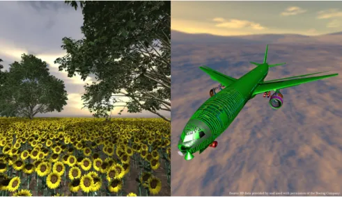
It does not, however, mean that rasterization is always faster than ray tracing: there are cases where ray tracing outperforms rasterization. Consider, for example, a very big polygonal model: using a spatial subdivision to accelerate ray–polygon intersection, ray tracing computational complexity grows logarithmically with the increasing number of polygons. Computational complexity of rasterization, on the other hand, will grow linearly with the increasing number of polygons. Consequently, rasterization may outperform ray tracing on smaller scenes, because it typically needs less computations per polygon; however, as the number of polygons grows, so does the computational cost, because all polygons need to be rasterized before performing the depth test. It is demonstrated in works of Wald et. al [1] [20], where they used ray tracing to visualize

(28)

Figure 2.1: Sunflowers (1 billion triangles) and Boeing 777 (370 million triangles) from the works of Wald et al. [1], [2]. Scenes of such complexity are much easier to render with ray tracing than with rasterizing.

scenes like a very detailed model of a Boeing 777 aircraft (350 million triangles) or a sunflower field (about 1 billion triangles) (see Fig. 2.1). Another example where ray tracing would probably be faster is a scene with reflective object: with rasterization, it would be required to render the entire scene (or at least big portions of the entire scene) from a different perspective for every reflective surface to generate reflections (even in the very limited way that rasterization allows). For more details on computational complexity of ray tracing see, for example, the work of Reif et al. [21].

Theory and implementation details

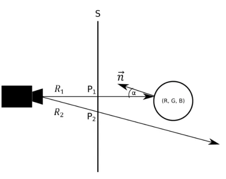
Ray tracing in its simplest form (often called ”ray casting” nowadays to distinguish it from recursive ray tracing) works as follows (Fig. 2.2):

• An imaginary ray is cast from the ”camera” towards the 3D scene, passing through a particular pixel coordinates on the computer monitor.

• The ray is checked for intersection with every object of the 3D scene.

(29)

Figure 2.2: Scheme of simple, non–recursive ray tracing. Two rays are shown: R1hitting andR2missing the scene object (the circle). Solid line S represents the screen. Using cosine law, the screen point P1 is going to have the same (R, G, B) color as the object material, multiplied by cosα, whereαis the angle between

−R1 and the object’s surface normal at the hit point.

• If no intersection is found, a background color value is assigned to the screen pixel (for example, black color).

• If one or more intersections are found, the closest intersection point is determined. With the ray represented as an origin pointP_oand a direction vector−→

V, that is the intersection pointP=P_o+t−→ V for whichtis minimal.

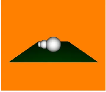
• Color for the screen pixel is calculated based on the material properties of the intersected object as well as any other data, such as the distance from the camera, the surface normal at the intersection point and so on (Fig. 2.3).

With this scheme, only ambient illumination can be used, with no additional light sources and no shadows.

Simple (e. g. absolute) transparency can be used, but light attenuation, shadows, reflection and refraction cannot.

(30)

Figure 2.3: Simple non–recursive ray tracing of a green plane and three white spheres. Orange is used as the background color, and cosine law is used for shading.

Figure 2.4: Shadow rays in recursive ray tracing. Primary rays are cast from the camera, spawning secondary shadow rays, originating at their points of intersection with the ground plane and directed towards the light source L. Where these shadow rays are blocked by scene objects and unable to reach the light source, a shadow is created.

(31)

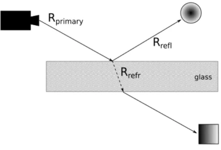
Figure 2.5: Reflection and refraction rays in recursive ray tracing. Primary rayR_primary spawns two secondary rays: a reflection rayRref land a refraction rayRref r. Possibly intersecting other scene objects, these ray bring back some additional color information, which is then blended according to the selected coloring scheme, creating reflection and refraction.

Recursive ray tracing, introduced by Whitted [16], extends the ray casting scheme described above with possibility of casting secondary rays from the intersection points. Those rays include:

• Shadow rays, cast towards every light source in the scene (see Fig. 2.4).

• Reflection rays, cast if the material at the current intersection point has reflective properties (see Eq.

2.9 below).

• Refraction rays, cast if the material at the current intersection point is not completely opaque. Such rays change direction when the material changes its refractive index (see Eq. 2.12) and can get attenuated, if the material is not completely transparent (Eq. 2.14).

Each secondary ray in its turn can produce more secondary rays when intersecting a scene object, although for practical reasons a recursion limit is usually imposed. With recursive ray tracing, different kinds of additional light sources can be used. Shadows, partial transparency, reflection and refraction can be modeled

(32)

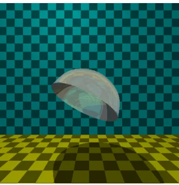
Figure 2.6: Recursive ray tracing of a semi–transparent colorless bell and two planes with procedural check- ered textures. Reflection, refraction and light attenuation can be seen on the bell, and a shadow effect — on the floor underneath it.

in a very unified and general way (Fig. 2.6). Visual effects such as caustics still cannot be modeled, requiring more advanced techniques, such as photon mapping.

For shadowing we used Blinn–Phong shading model with the following parameters:

• k_a, which is an ambiend reflection constant

• k_d, which is a diffuse reflection constant

• ks, which is a specular reflection constant

• alpha, which is a material shininess constant

Formlight sources, the illumination of each surface pointIp is then defined as

Ip=kaia+ X

m∈lights

(kd( ˆLm·N)iˆ m,d+ks( ˆN·Hˆ)^αim,s) (2.7)

where

(33)

• Lˆmis the direction vector from the surface point towards each of themlight sources

• Nˆ is the surface normal at the point

• im,dandim,s are diffuse and specular RGB color intensities of the light sources

• i_a is the intensity of the ambient light

Hˆ is defined as

Hˆ = L+V

kL+Vk, (2.8)

where Lis a direction vector from the surface point towards the light source andV — from the surface point towards the camera.

To generate objects reflections, used in jellyfish rendering, reflectivity constant k_r was added to the material parameters, and recursion limit r_c and importance cutoff y_c — to the ray parameters. Primary rays start with their recursion counterr= 0 and their importancey= 1. If the following three conditions are satisfied for any rayRi

• r < r_c

• y≥y_c

• kr>0 at the hit point

then a secondary rayR_i+1 is cast with the following parameters

ˆ

v_i+1= ˆv_i−2 ˆN_i( ˆN_i·vˆ_i) r_i+1=r_i−1

yi+1=yiY⁰

(2.9)

where ˆv is the vector direction, ˆN is the surface normal at the hit point andY⁰ is a luminance constant, defined as

(34)

Y⁰ =Yntsc·kr, (2.10)

whereY_ntsc={0.299,0.587,0.114}is a constant color vector defined by NTSC standard. Each subsequent ray makes its contribution to the resulting color, which is

Ir=kr×Ip, (2.11)

where I_p is the illumination, calculated according to equation 2.7.

To simulate refraction of light occurring at the jellyfish boundaries, we used Schlick’s approximation of Fresnel equations, which is

R(θ) =R0+ (1−R0)(1−cosθ)⁵ R0=

n1−n2

n₁+n₂

²

(2.12)

where θis the angle between the direction of incoming light, n₁ andn₂ are refractive indices of the two materials at the boundary of which the refraction occurs. R(θ) determines what part of the incoming light intensity gets reflected off the boundary in the reflection direction, while the rest travels through the material with refractive indexn2, and its direction is determined by Snell’s law:

sinθ1

sinθ₂ =n2

n₁ (2.13)

In our case, there were two translucent materials: the sea water and the mesoglea of jellyfish. The refraction index of sea water varies slightly with the water temperature, salinity and for different light wave lengths, but in our work we kept it constant and equal to 1.33. Jellyfish mesoglea may have varying refraction index, depending on the species, and in our work we used values in the 1.0–1.4 interval.

Similarly to the reflection, secondary refraction rays are cast recursively, their contribution to the final illumination value is accumulated. Travelling through materials, rays get attenuated according to Beer–

Labmert law, which is

(35)

T=e^−µl, (2.14)

where µis the attenuation coefficient andl is the distance travelled by the ray through the material.

Using recursive ray tracing for purposes other than optical effects

The usage of ray tracing in computer graphics is not limited to visualization. It is used, for example, for collision detection: similarly to casting camera rays and checking their intersection with scene objects in order to visualize them, it is possible to cast rays off the surface of a moving scene object in order to check if the object is about to collide with another object. In this work, while using whitted–style ray tracing for visualization, we recursively cast additional ”probe” rays to visually correct problems left unsolved by underlying physical simulation.

2.5 Spatial hierarchies

Space partitioning is widely used in this work. As rendering scenes tend to be quite large in terms of polygon count, naive approach to calculating ray–polygon intersection, which is testing every ray for intersection with every polygon, is too slow for real–time visualization. That is also true for collision detection and for particle interaction in fluid simulation in Chapter 3. We used HLBVH2 (see [22] for details) for recursive ray tracing, andk-d tree to quickly search for neighbouring particles in the MPS fluid simulation in 2D. In both cases, that changed the complexity fromO(n²) toO(nlogn).

2.6 GPU acceleration

Graphics processing units (GPU) typically have much higher number of processing cores than CPUs, although the cores themselves are less computationally powerful. This makes GPUs to be much faster than CPUs for some tasks, most noticeably, computer graphics–related, such as polygon rasterizing and image processing, where a single program (often called ”shader” or ”kernel”) performing relatively simple calculation can

(36)

be executed simultaneously on a large array of data. While originally GPUs could only accept graphical data from CPUs, process it and pass forward to a display, in later GPUs two–way interaction became available, with data coming back from the GPU to the CPU. This made general purpose GPU programming (GPGPU) possible. While polygon rasterizing was supported even in earliest GPUs, GPU–accelerated ray tracing became possible only using later GPGPU features, and it does not benefit from GPU acceleration as much as rasterizing does. That is due to more divergent control flow in ray tracing: while with rasterizing a GPU operates on polygon vertices, performing exactly same operations on each one, with ray tracing it has to operate on rays, performing different sets of operations depending on whether the ray misses or hits an object, gets reflected/refracted, and so on. Still, 1–2 orders of magnitude speedup can be achieved, compared to the CPU ray tracing, depending on the complexity of the computational model.

2.7 Conclusion

In this chapter we outlined our technique for deformable body visualization, based on simplified physics, RBF space mapping and special case of recursive ray tracing. While we were using PhysX in our particular implementation, any physical simulation software can be used instead, its results taken, modified with RBFs and visualized with ray tracing. Perhaps the biggest drawback of our method is its lack of generality: while it has shown good result for practically important cases, such as marine animal simulation and multiple garment visualization, it will not work for every imaginable case of deformable body, or even for some more exotic sets of garment. We further discuss these limitations in chapters 3–5. Our heavy reliance on recursive ray tracing, which is not the fastest rendering method known to mankind, can be considered a drawback as well. However, complex physical interaction, typically used for the tasks we were trying to accomplish, are usually much slower, and as we replace a part of those physical interactions with our ray tracing, it results in significant saving in required computations. Finally, an advantage of our method is that, however it can be used together with an iterative physical simulation, it is itself not iterative, with all the computations done in a single pass, so there is no need to wait for an iteration to complete in order to start the next iteration.

(37)

Chapter 3

Artificial jellyfish: optimization of deformable shape

3.1 Introduction

Jellyfish are the earliest known animals to use muscle power for swimming [23]. They swim by contracting and expanding their mesogleal bells. The swimming muscles contract to expel a portion of water rearward out of the subumbrellar cavity, thus generating a thrust force to move the animal forward. The bell is refilled when it restores its shape after deformation it received during the thrust phase. The bell consists of a fiber-reinforced composite material called ”mesoglea”. The elastic characteristics of the mesogleal tissue were studied, for example, by Megill et al. [24]

The contractile muscle fibers of the medusae are only one cell layer thick, so the forces that they can produce do not scale favorably with the increasing medusa size. For a medusa with the bell of diameterD, the mass of water that needs to be expelled from within the bell scales as D³, while the muscle force only scales asD¹. Therefore the force required for jet propulsion increases with the animal size more rapidly than the available physiological force [23]. Thus, the swimming performance may change dramatically with the increase of the medusan body size, and it is impossible to predict the optimal swimming parameters based

(38)

on the geometric and kinematic similarity.

The physics of jellyfish swimming is not well understood. Existing animation techniques use combinations of sinusoidal curves to specify the deformations. However, it is important for animation to achieve a realistic movement depending on the size and shape of a bell. We assume that ”realistic” also means ”optimal”, as the movements of the real jellyfish were ”optimized” by the process of natural evolution, and we, therefore, would be able to find realistic movements for an artificial 3D model of jellyfish by means of artificial evolution. Other applications, such as computational biology, soft robotics and development of new propulsion techniques can benefit from development of a generalized model of jellyfish swimming.

In this thesis we present a system for finding optimal swimming parameters for jellyfish models, based on our previous work where we studied vortex simulation for jellyfish [25]. The system consists of two main parts: simulated swimming and motion optimization. We introduce a simple technique based on radial basis functions (RBF) to model deformations of the jellyfish bell and a particle-gridless hybrid method for the analysis of incompressible flows. We modeled the interaction between the fluid particles and the surface of the bell in a form of elastic collision and reflection of the fluid particles off the boundary surface. The swimming efficiency was estimated for the bell and its particular movement specified by a set of control points.

Genetic algorithms were used to find the optimal swimming pattern. To the best of our knowledge, this is the first work where the optimal swimming parameters for the jellyfish movement were found by solving the optimization problem. Throughout the paper we refer to two other paper concerning computational simulation of jellyfish ([26] and [27]), but neither of those employs any numerical optimization.

The remainder of this chapter is divided into 7 sections. In section 3.2 we discuss related work. We describe our approach in sections 3.3 to 3.5 and outline the algorithm in section 3.6. In section 3.7 we outline the specifics of our prototype implementation and report of the experimental results, and in section 3.8 we conclude the chapter and explain some limitations and possible directions of future work.

(39)

3.2 Related work

Studies of real life jellyfish

Experimental studies, including dye injection, filming and analyzing the resulting flow, indicate that smaller prolate medusae create strong jets during their bell contraction stage. Bigger oblate medusae, however, produce substantially less distinct jets and broad vortices at the bell margins. A hypothesis proposed by Colin and Costello [28] [23] [29] [30] is that oblate species are using their bell’s margins as ”paddles”, thus utilizing a paddling, or rowing, mode of swimming. According to the model presented by Dabiri et al. [23], big oblate medusae are not capable of swimming via jet propulsion. There is, however, a study of McHenry and Jed [31] which suggests that the jetting model still provides more accurate approximation of swimming in oblate jellyfish.

The flow generated by oblate medusa’s pulsatile jets consists mostly of radially symmetric rotating currents called vortex rings. To better understand the vortex formation and their effect on swimming performance, numerous experimental studies of real live jellyfish were performed [28] [23] [31] [32] [29] [30].

Researches using mechanical jet generators demonstrate that there is a physical limit – called the ”vortex formation number” – for the maximum size of the vortex rings. Once this number is reached, no bigger vortex formation is possible, and the extra water creates a trailing current behind the vortex. The energy cost for generating this current is higher than that of creating the vortex ring, so it is optimal to generate the largest possible vortex without any trailing current [29]. Both thrust and efficiency increase in direct proportion with vortex ring volume [30]. Lipinski and Mohseni [26] used digitized motions of two real hydromedusae to computationally simulate the flows. Their results confirm the hypothesis proposed by Colin and Costello and demonstrate that distinct type of jellyfish (”jetting” and ”paddling”) produce substantially different kinds of vortices.

(40)

Fluid-solid interaction

M¨uller et al. proposed a particle-based method for interaction of fluids with deformable solids [33]. In their method they model the exchange of momentum between Lagrangian particle-based fluid model and solids represented by polygonal meshes with virtual boundary particles to model the solid-fluid interaction.

Lipinski and Mohseni [26] used digitized motions of two real hydromedusae to computationally simulate the flows. They used a new arbitrary Lagrangian-Eulerian method with mesh following the boundary between the fluid and the jellyfish body.

Yoon et al. presented a particle-gridless hybrid method for the analysis of incompressible flows [34].

Their numerical scheme included Lagrangian and Eulerian phases. The moving-particle semi-implicit method (MPS) was used for the Lagrangian phase, and a convection scheme based on a flow directional local grid was developed for the Eulerian phase.

Chentanez et al. presented a method for simulating the two-way interaction between fluids and deformable solids [35]. The fluids were simulated using an incompressible Eulerian formulation where a linear pressure projection on the fluid velocities enforces mass conservation, whereas elastic solids were simulated using a semi-implicit integrator implemented as a linear operator applied to the forces acting on the nodes in Lagrangian formulation.

Hirato et al. proposed a method for generating animations of jellyfish with tentacles [36]. They used a simplified computational model based on the MPS method to simulate the fluid. Their work is mainly focused on visually plausible modeling of tentacles.

Rudolf and Mould created a system for physically-based animation of jellyfish [27]. Their approach may look very similar to ours, as they also exploited the radial symmetry, simulating only a 2D cross-section, and then creating a 3D bell for the visualization. The main difference between the approach proposed in [27] and the one discussed in this paper is that Rudolf and Mould did not employ any optimization, instead assigning a visually plausible set of parameters manually, by trial and error. They used a spring-mass system to represent the body of a jellyfish and a grid-based immersed boundary method for fluid-solid coupling. As

(41)

they note in their work, there is still very little knowledge about physical properties of real jellyfish. Thus, we didn’t feel necessary to employ something as complex as a spring-mass system, since the actual physical accuracy of the model would still be uncertain. Moreover, modeling a multi-layered structure of the jellyfish bell with only one layer of springs attached directly to the opposite sides of the bell does not look realistic.

Some fugures from [27] demonstrate drastic change of both area and linear size of the umbrella cross-section during the contraction, something we failed to observe in real species, such as presented in experiments of Colin and Costello [30]. Instead of a spring-mass system, we use a simpler approach, with the umbrella of the jellyfish represented in 2D as two spline curves, deformed by RBFs. Instead of a grid-based method, for fluid simulation we used a particle-based method [34] with elastic collision and reflection of the fluid particles off the boundary surface to prevent fluid leaking across the boundary. Finally, [27] employs a very primitive visualization technique, an issue we were trying to address with a GPU-based parallel ray tracer, capable of representing transparency, reflectivity and venous structure.

Optimization

The problem was studied by many researchers from the computer graphics and animation community, but we have no room for the comprehensive referencing, so we will mention only a few we found most relevant to out work.

Sims was one of the pioneers of artificial evolution. In his work [37] he used genetic algorithms to create evolving images, textures, animations and plants, represented by procedural geometry, with human aesthetical selection instead of a fitness function. In [38] he used similar approach to artificially evolve both morphology and behavior of articulated (e. g. composed of rigid parts and connecting joints) creatures, which were evolved and trained to perform specific tasks, like walking, jumping, following a light source, competing for a ball with other creatures etc.

Terzopoulos et al. [39] modeled artificial fish as NURBS and spring-mass systems, using simulated annealing to find efficient moving patterns. Based on simulated sensory input, their fish could learn complex group behaviour, such as schooling, mating etc.