R ESEARCH I NSTITUTEFOR M ATHEMATICAL S CIENCESKYOTOUNIVERSITY,Kyoto,Japan BySakieSUZUKIMarch2011 Ontheuniversal sl invariantofboundarybottomtangles RIMS-1716

(1)

RIMS-1716

On the universal sl

2

invariant of boundary bottom tangles

By

Sakie SUZUKI

March 2011

R _ESEARCH I NSTITUTE FOR M ATHEMATICAL S _CIENCES

(2)

On the universal sl ₂ invariant of boundary bottom tangles

Sakie Suzuki

^∗

March 11, 2011

Abstract

The universalsl2invariant of bottom tangles has a universality property for the colored Jones polynomial of links. Habiro conjectured that the universalsl2invariant of boundary bottom tangles takes values in certain subalgebras of the completed tensor powers of the quantized enveloping algebraUh(sl2) of the Lie algebrasl2. In the present paper, we prove an improved version of Habiro’s conjecture. As an application, we prove a divisibility property of the colored Jones polynomial of boundary links.

1 Introduction

In the 80’s, Jones [9] constructed a polynomial invariant of links. After that, Reshetikhin and Turaev [20] defined an invariant of framed links whose components are colored by finite dimensional representations of a ribbon Hopf algebra. The colored Jones polynomial is the Reshetikhin-Turaev invariant of links whose components are colored by finite dimensional representations of the quantized enveloping algebraUh(sl2).

The universal invariant associated with a ribbon Hopf algebra is an invariant of framed links and tangles which are not colored by any representations, see Hennings [8], Lawrence [15, 14], Reshetikhin [20], Ohtsuki [19], Kauﬀman [10], and Kauﬀman and Radford [11]. The universal invariant has the universality property for the Reshetikhin-Turaev invariant. By the universalsl2invariant, we mean the universal invariant associated withUh(sl2). In particular, one can obtain the colored Jones polynomial from the universalsl2 invariant.

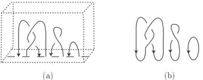
Abottom tangle is a tangle consisting of arc components in a cube such that each boundary point is on the bottom line, and the two boundary points of each component are adjacent to each other, see Figure 1 (a) for example. We can deﬁne the closure link of a bottom tangle, see Figure 1 (b). For each link L, there is a bottom tangle whose closure isL. In [4], Habiro studied the universal invariant of bottom tangles associated with a ribbon Hopf algebra, and in [6], he studied the universalsl2 invariant in detail.

The universalsl2invariant ofn-component bottom tangles takes values in the completed n-fold tensor power Uh(sl2)^⊗^ˆⁿ of Uh(sl2). By using bottom tangles, we can restate the universality of the universalsl2invariant: the colored Jones polynomial of a linkLis obtained from the universalsl2invariant of a bottom tangle whose closure isL, by taking the quantum traces associated with the representations attached to the components of links (cf. [4]).

We are interested in relationships between the algebraic properties of the colored Jones polynomial and the universalsl2invariant and the topological properties of links and bottom tangles.

∗Research Institute for Mathematical Sciences, Kyoto University, Kyoto, 606-8502, Japan. E-mail address:

[email protected]

(3)

Figure 1: (a) A bottom tangleT (b) The closure link ofT

Figure 2: A boundary bottom tangle

Eisermann [2] proved that the Jones polynomial of ann-component ribbon link is divisible by the Jones polynomial of then-component unlink. This result is generalized to links which are ribbon concordant to boundary links by Habiro [7]. Habiro [6] proved that the universal sl₂ invariant of n-component, algebraically-split, 0-framed bottom tangles takes values in certain small subalgebras of the completed tensor powers of U_h(sl₂), and gave a divisibility property of the colored Jones polynomial of algebraically-split, 0-framed links.

In [21], the present author proved an improvement of Habiro’s result for algebraically-split, 0-framed bottom tangles, in the special case ofribbon bottom tangles and ribbon links.

In the present paper, we study the universalsl₂invariant of boundary bottom tangles. A bottom tangle is called boundary if its components admit mutually disjoint Seifert surfaces, see Figure 2 for example. We can obtain each boundary link from a boundary bottom tangle by closing. Habiro [6] conjectured that the universalsl2invariant of boundary bottom tangles takes values in certain subalgebras of the completed tensor powers ofUh(sl2). We prove an improved version of Habiro’s conjecture (Theorem 1.2).

1.1 Main result

The quantized enveloping algebraUh=Uh(sl2) is anh-adically completedQ[[h]]-algebra (see Section 2.2 for the details). We setq= exph.

Habiro [6] proved that the universal sl2 invariant JT of an n-component, algebraically- split, 0-framed bottom tangleT is contained in the Z[q, q⁻¹]-subalgebra ( ˜Uqêv)^⊗^˜ⁿ ofU_h^⊗^ˆⁿ. In [21], we defined another Z[q, q⁻¹]-subalgebra ( ¯U_qêv)ˆ^⊗^ˆⁿ ⊂ ( ˜Uqêv)^⊗^˜ⁿ, and prove the following theorem. (See Section 2.3 for the definition of ¯U_qêv, and see Sections 6.1–6.4 for the definition of the completion ( ¯U_qêv)ˆ^⊗^ˆⁿ of ( ¯U_qêv)^⊗ⁿ.)

Theorem 1.1 ([21]). Let T be an n-component ribbon bottom tangle with 0-framing. Then we have J_T ∈( ¯U_q^ev)ˆ^⊗^ˆⁿ.

The main result of the present paper is the following.

(4)

Theorem 1.2. Let T be an n-component boundary bottom tangle with 0-framing. Then we haveJ_T ∈( ¯U_q^ev)ˆ^⊗^ˆⁿ.

Remark 1.3. Habiro [6, Conjecture 8.9] conjectured Theorem 1.2 with ( ¯U_qêv)ˆ^⊗^ˆⁿ replaced with the Z[q, q⁻¹]-subalgebra ( ¯U_qêv)˜^⊗^˜ⁿ, which includes ( ¯U_qêv)ˆ^⊗^ˆⁿ. We do not know whether the inclusion ( ¯U_qêv)ˆ^⊗^ˆⁿ ⊂( ¯U_qêv)˜^⊗^˜ⁿ is proper or not. The definition of our algebra ( ¯U_qêv)ˆ^⊗^ˆⁿ appears to be more natural.

Since every 1-component bottom tangle is boundary, Theorem 1.2 forn= 1 gives a possible improvement of the following theorem.

Theorem 1.4 (Habiro). Let T be an 1-component bottom tangle with 0-framing. Then we haveJT ∈( ¯U_q^ev)˜.

Theorem 1.4 follows from [6, Theorem 4.1] and the equalities Inv( ˜Uqêv) =Z( ˜Uqêv) =Z(( ¯U_qêv)˜),

which is implicit in [5, Section 9]. Here, for a subset X ⊂ Uh, we denote by Inv(X) the invariant part ofX, and byZ(X) the center ofX.

If we use the one-to-one correspondence described in [4, Section 13] between the set of bottom tangles and the set of string links, then we can deﬁne the Milnor ¯µinvariants [17, 18]

of a bottom tangle as that of the corresponding string link. See [3] for the Milnor ¯µinvariants of string links. In fact, all Milnor ¯µ invariants vanish both for ribbon bottom tangles and boundary bottom tangles. It is natural to expect the following conjecture.

Conjecture 1.5. If T be an n-component bottom tangle with 0-framing with vanishing all Milnor µ¯ invariants, then we haveJT ∈( ¯U_q^ev)ˆ^⊗^ˆⁿ.

The converse of Conjecture 1.5 is also open.

1.2 Application to the colored Jones polynomial

We give an application (Theorem 1.6) of Theorem 1.2 to the colored Jones polynomial of boundary links. This result is parallel to the result for ribbon links [21].

We use the following q-integer notations:

{i}q =qⁱ−1, {i}q,n={i}q{i−1}q· · · {i−n+ 1}q, {n}q! ={n}q,n, [i]q ={i}q/{1}q, [n]q! = [n]q[n−1]q· · ·[1]q,

·i n

¸

q

={i}q,n/{n}q!, fori∈Z, n≥0.

For m ≥ 1, let V_m denote the m-dimensional irreducible representation of U_h. Let R denote the representation ring ofU_hoverQ(q¹²), i.e., Ris theQ(q¹²)-algebra

R= Span

Q(q¹2){V_m |m≥1}

with the multiplication induced by the tensor product. It is well known thatR=Q(q¹²)[V2].

(5)

Forl≥0, set

Pl=

l−1

Y

i=0

(V2−qⁱ⁺¹² −q⁻ⁱ⁻¹²)∈ R, P˜_l⁰= q¹²^l

{l}q!Pl∈ R,

which are used in [6] to construct the uniﬁed Witten-Reshetikhin-Turaev invariants for integral homology spheres. We denote by J_{L; ˜}_P0

l1,...,P˜⁰

ln

the colored Jones polynomial of L with ith component Li colored by ˜P_l⁰

i. Habiro proved that Theorem 1.2 implied the following result.

Forl≥0, letIl denote the ideal inZ[q, q⁻¹] generated by{l−k}q!{k}q! fork= 0, . . . , l.

Theorem 1.6([6, Conjecture 8.10]). LetLbe ann-component boundary link with0-framing.

Forl1, . . . , ln≥0, we have J_{L; ˜}_P0

l1,...,P˜_ln⁰ ∈ {2lj+ 1}q,l_j+1

{1}q

I_l₁· · ·Iˆ_l_j· · ·I_l_n,

wherej is an integer such thatl_j = max{l_i}1≤i≤n, andIˆ_l_j denotes the omission ofI_l_j. Remark 1.7. Form≥1, let Φ_m(q) =Q

d|m(q^d−1)^µ(^m^d⁾∈Z[q] denote themth cyclotomic polynomial, whereQ

d|mdenotes the product over all the positive divisorsdofm, andµis the M¨obius function. It is not diﬃcult to prove that forl≥0,Ilis contained in the principal ideal inZ[q] generated byQ

mΦm(q)^f(l,m)withf(l, m) = max{0,¥_l+1

m

¦−1}, where, forr∈Q, we denote bybrcthe largest integer smaller than or equal tor.

Theorem 1.6 is an improvement in the special case of boundary links of the following result.

Theorem 1.8 (Habiro [6, Theorem 8.2]). Let L be an n-component, algebraically-split link with0-framing. Forl₁, . . . , l_n ≥0, we have

J_{L; ˜}_P0

l1,...,P˜_ln⁰ ∈ {2lj+ 1}q,l_j+1

{1}q

Z[q, q⁻¹].

1.3 Examples

LetTB be the Borromean bottom tangle depicted in Figure 3 (a), whose closure is the Bor- romean rings. Since we haveJT_B ∈/( ¯U_q^ev)ˆ^⊗^ˆ³(cf. [21]), it follows from Theorem 1.2 that the Borromean rings is neither boundary nor ribbon, as is well known.

More generally, for n ≥ 3, let Mn be Milnor’s n-component Brunnian link depicted in Figure 3 (b). Note that M3 is the Borromean rings. Since there is a non-trivial Milnor ¯µ invariant ofMn of lengthn(cf. [17]),Mn is neither boundary nor ribbon. We can prove this fact also from Theorem 1.6 and

J_M

n; ˜P₁⁰,...,P˜₁⁰ = (−1)ⁿ⁻²q⁻²ⁿ⁺⁴Φ1(q)ⁿ⁻²Φ2(q)ⁿ⁻²Φ3(q)Φ4(q)ⁿ⁻³

∈/Φ₁(q)ⁿΦ₂(q)Φ₃(q)Z[q, q⁻¹], which we will prove in a forthcoming paper [22].

(6)

・・・

Figure 3: (a) Borromean rings (b) Milnor’s linkM_n

Figure 4: (a) A tangle (b) The framing on the boundary

1.4 Organization of paper

The rest of the paper is organized as follows. Section 2 contains preliminary results about bottom tangles, the quantized enveloping algebraUh, and the universalsl2invariant of bottom tangles. In Section 3, we recall from [6] Habiro’s formula for the universal sl2 invariant of boundary bottom tangles, and then give a modiﬁcation of his formula. In Sections 4, 5, and 6, we prove Theorem 1.2.

2 Preliminaries

In this section, we recall basic things about bottom tangles, the universal enveloping algebra U_h, and the universalsl₂invariant of bottom tangles.

2.1 Bottom tangles and boundary bottom tangles

Atangle (cf. [12]) is the image of an embedding

³a^m [0,1]

´t³aⁿ S¹

´

,→[0,1]³,

withm, n≥0,whose boundary is on the two lines [0,1]× {¹₂} × {0,1}on the bottom and the top of the cube, see Figure 4 (a) for example. We equip the image with both an orientation and a framing. Here, at each boundary point, the framing is ﬁxed on the lines [0,1]× {¹₂} × {0,1} as in Figure 4 (b), where the thin arrows represent the strands of the tangle, and the thick arrows represent the framing.

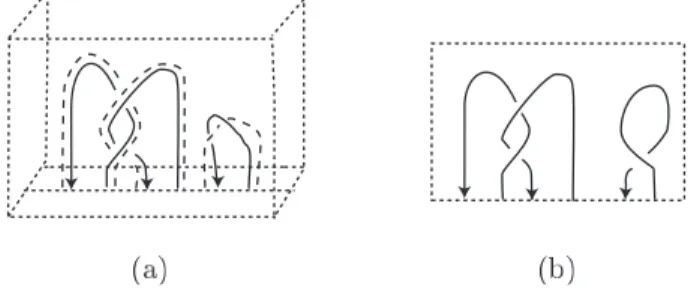
A bottom tangle (cf. [4, 6]) is a tangle consisting of arc components such that each boundary point is on the line [0,1]× {¹₂} × {0}on the bottom, and the two boundary points of each component are adjacent to each other. We give a preferred orientation of the tangle so that each component runs from its right boundary point to its left boundary point. For example, see Figure 5 (a), where the dotted lines represent the framing. We draw a diagram of a bottom tangle in a rectangle assuming the blackboard framing, see Figure 5 (b).

(7)

Figure 5: (a) A 3-component bottom tangleT (b) A diagram ofT

For eachn≥0, letBTn denote the set of the ambient isotopy classes, relative to boundary points, ofn-component bottom tangles.

Theclosure link cl(T) of a bottom tangleT is deﬁned as the link in R³ obtained fromT by closing, see Figure 1 again. For eachn-component linkL, there is ann-component bottom tangle whose closure is L. For a bottom tangle, we can deﬁne its linking matrix as that of the closure link.

A Seifert surfaceof knotK is a compact, connected, orientable surfaceF in R³bounded byK. Ann-component linkL=L1∪ · · · ∪Lnis calledboundary if it hasnmutually disjoint Seifert surfacesF1, . . . , Fn in R³such thatLi boundsFi fori= 1, . . . , n.

For a 1-component bottom tangle T ∈BT₁, there is a knot K_T =T ∪γ ∈[0,1]³, where γ is the line segment in the bottom [0,1]× {¹₂} × {0}such that ∂γ =∂T. ASeifert surface of a 1-component bottom tangleT is a Seifert surface of the knotK_T contained in [0,1]³. A bottom tangleT =T₁∪· · ·∪T_nis calledboundary if it hasnmutually disjoint Seifert surfaces F₁, . . . , F_nin [0,1]³such thatK_T_iboundsF_ifori= 1, . . . , n. For example, see Figure 2 again.

Obviously, for each boundary linkL, there is a boundary bottom tangle whose closure isL.

2.2 Quantized enveloping algebra U

_h

We recall the deﬁnition of the universal enveloping algebraU_h(sl₂) of the Lie algebrasl₂, and its ribbon Hopf algebra structure. We follow the notations in [6].

We denote byU_h=U_h(sl₂) theh-adically completeQ[[h]]-algebra, topologically generated byH, E,andF, deﬁned by the relations

HE−EH = 2E, HF−F H =−2F, EF −F E= K−K⁻¹ q^1/2−q⁻^1/2, where we set

q= exph, K=q^H/2= exphH 2 .

We equipUhwith the topologicalZ-graded algebra structure such that degE= 1, degF =

−1, and degH = 0. For a homogeneous elementxofUh, the degree ofxis denoted by|x|. There is a complete ribbon Hopf algebra structure on Uhas follows. The comultiplication

∆ : Uh→Uh⊗ˆUh, the counitε: Uh→Q[[h]], and the antipodeS: Uh→Uhare given by

∆(H) =H⊗1 + 1⊗H, ε(H) = 0, S(H) =−H,

∆(E) =E⊗1 +K⊗E, ε(E) = 0, S(E) =−K⁻¹E,

∆(F) =F⊗K⁻¹+ 1⊗F, ε(F) = 0, S(F) =−F K.

(8)

Set

D=q¹⁴^H^⊗^H= exp¡h

4H⊗H¢

∈U_h^⊗^ˆ², (1)

F˜⁽ⁿ⁾=FⁿKⁿ/[n]q!∈Uh, (2)

e= (q^1/2−q⁻^1/2)E∈Uh, (3)

forn≥0. The universalR-matrix and its inverseR^±¹∈Uh⊗ˆUh are given by R=DX

n≥0

q¹²ⁿ⁽ⁿ⁻¹⁾F˜⁽ⁿ⁾K⁻ⁿ⊗eⁿ, R⁻¹=D⁻¹X

n≥0

(−1)ⁿF˜⁽ⁿ⁾⊗K⁻ⁿeⁿ. We haveR^±¹=P

n≥0α^±_n ⊗β_n^±, where forn≥0,we set formally αn⊗βn( =α⁺_n ⊗β_n⁺) =D

³

q¹²ⁿ⁽ⁿ⁻¹⁾F˜⁽ⁿ⁾K⁻ⁿ⊗eⁿ

´ , α_n⁻⊗β_n⁻=D⁻¹

³

(−1)ⁿF˜⁽ⁿ⁾⊗K⁻ⁿeⁿ

´ .

Note that the right hand sides are inﬁnite sums of tensors of the form asx⊗ywithx, y∈Uh. We denote them byα^±_n ⊗β_n^± for simplicity.

The ribbon element and its inverse r^±¹∈Uh are given by r=X

n≥0

α⁻_nK⁻¹β_n⁻=X

n≥0

β_n⁻Kα⁻_n, r⁻¹=X

n≥0

α_nKβ_n =X

n≥0

β_nK⁻¹α_n. We use a notationD=P

D⁰⊗D⁰⁰. We use the following formulas.

XD⁰⁰⊗D⁰=D, (4)

(∆⊗1)D=D23D13, (1⊗∆)D=D13D12, (5)

(ε⊗1)(D) = 1 = (1⊗ε)(D), (6)

(1⊗S)D=D⁻¹= (S⊗1)D, (7)

D(1⊗x) = (K^|^x^|⊗x)D, D(x⊗1) = (x⊗K^|^x^|)D, (8) whereD₁₃=P

D⁰⊗1⊗D⁰⁰,D₂₃= 1⊗D, D₁₂=D⊗1, andx∈U_h homogeneous.

2.3 Subalgebras of U

_h

In this section, we recall from [6] subalgebrasU_Z_,q,U¯_q and ¯U_q^evofU_h. Recall from (2) and (3) the deﬁnitions of ˜F⁽ⁿ⁾∈U_hande∈U_h, respectively. Similarly, set

E˜⁽ⁿ⁾= (q⁻^1/2E)ⁿ/[n]q!∈Uh, f = (q−1)F K ∈U_h,

forn≥0.

Let U_Z,q denote the Z[q, q⁻¹]-subalgebra of Uh generated by K, K⁻¹,E˜⁽ⁿ⁾, and ˜F⁽ⁿ⁾ for n≥1.

Let ¯Uq denote theZ[q, q⁻¹]-subalgebra ofU_Z,q generated byK, K⁻¹, eandf. Let ¯U_q^ev be theZ[q, q⁻¹]-subalgebra of ¯Uq generated byK², K⁻², eandf.

(9)

Remark 2.1. Set [i] = _q^q_1/2^i/2⁻₋^q_q^−i/2_−1/2 for i∈ Z and [n]! = [n]· · ·[1] for n≥0. Let U_Z be the Z[q^1/2, q⁻^1/2]-subalgebra ofU_hgenerated byK, K⁻¹, E⁽ⁿ⁾=Eⁿ/[n]!, andF⁽ⁿ⁾=Fⁿ/[n]! for n≥1 (Lusztig’s integral form, cf. [16]). We have

U_Z=U_Z,q⊗_Z[q,q⁻¹]Z[q^1/2, q⁻^1/2].

Let ¯U denote theZ[q^1/2, q⁻^1/2]-subalgebra ofUh generated byK, K⁻¹, (q^1/2−q⁻^1/2)E, and (q^1/2−q⁻^1/2)F (cf. [1]). We have

U¯ = ¯U_q⊗_Z[q,q⁻¹]Z[q^1/2, q⁻^1/2].

There is a Hopf Z[q, q⁻¹]-algebra structure onU_Z,q inherited from Uh (cf. [16, 21]). We have

∆( ˜E^(m)) = Xm j=0

E˜^(m⁻^j)K^j⊗E˜^(j), (9)

∆( ˜F^(m)) = Xm j=0

F˜^(m⁻^j)K^j⊗F˜^(j), (10) S^±¹( ˜E^(m)) = (−1)^mq²¹^m(m^∓¹⁾K⁻^mE˜^(m), (11) S^±¹( ˜F^(m)) = (−1)^mq⁻¹²^m(m^∓¹⁾K⁻^mF˜^(m), (12) fori∈Z, m≥0. Similarly, there is a Hopf Z[q, q⁻¹]-algebra structure on ¯Uq inherited from Uh (cf. [1, 6]).

Let U_h⁰ denote the Cartan part of U_h, i.e., the subalgebra of U_h topologically generated byH. Let ¯U_q⁰ denote theZ[q, q⁻¹]-subalgebra of ¯U_q generated by K andK⁻¹. Let ¯U_q^{ev 0} be theZ[q, q⁻¹]-subalgebra of ¯Uq generated byK² andK⁻². We have

U¯_q⁰= ¯Uq∩U_h⁰, U¯_q^{ev 0}= ¯U_q^ev∩U_h⁰.

2.4 Adjoint action

In what follows, we use the following notations. Form≥0, let ∆^[m]: Uh→U_h^⊗^ˆ^mdenote the m-output comultiplication deﬁned by ∆^[0]=ε,∆^[1]= idU_h,and

∆^[m] = (∆⊗id^⊗_U^m⁻²

h )◦∆^[m⁻^1], form≥2. Forx∈Uh, m≥1, we write

∆^[m](x) =X

x(1)⊗ · · · ⊗x(m). Form₁, . . . , m_l≥0, set

∆^[m¹^,...,m^l^]= ∆^[m¹^]⊗ · · · ⊗∆^[m^l^]: U_h^⊗^ˆ^l→U_h^⊗^ˆ^m¹⁺^···^+m^l. (13) We use the left adjoint action ad : U_h⊗ˆU_h→U_h deﬁned by

ad(x⊗y) =x . y:=X

x₍₁₎yS(x₍₂₎), (14)

forx, y∈Uh. We use the following proposition.

(10)

, , , ,

Figure 6: Fundamental tangles, where the orientations of the strands are arbitrary

Figure 7: (a) A bottom tangleB∈BT2 (b) A diagram ofB (c) The labels which are put on the diagram ofB

Proposition 2.2 ([21, Proposition 3.2]). We have

U_Z_,q.U¯_qêv⊂U¯_qêv, U_Z_,q. KU¯_qêv⊂KU¯_qêv.

We also use a right action ad : Uh⊗ˆUh →Uh, which is the continuous Q[[h]]-linear map deﬁned by

ad(y⊗x) =y / x: =X

S⁻¹(x₍₂₎)yx₍₁₎,

=X

S⁻¹(x). y.

forx, y∈U_h. Proposition 2.2 implies the following.

Corollary 2.3. We have

U¯_qêv/ U_Z,q ⊂U¯_qêv, KU¯_qêv/ U_Z,q⊂KU¯_qêv.

2.5 Universal sl

₂

invariant of bottom tangles

For an n-component bottom tangle T = T1∪ · · · ∪Tn ∈ BTn, we deﬁne the universal sl2

invariantJT ∈U_h^⊗^ˆⁿ as follows ([19, 4]).

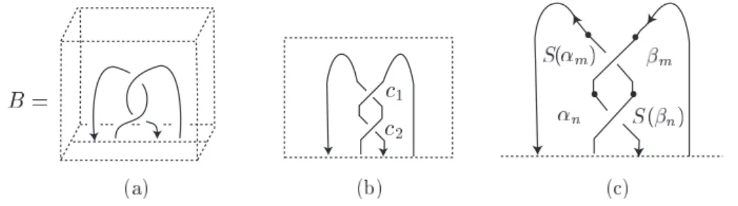
We choose and ﬁx a diagram of T obtained from the copies of the fundamental tangles depicted in Figure 6, by pasting horizontally and vertically. For example, for the bottom tangleB depicted in Figure 7 (a), we can take a diagram depicted in Figure 7 (b). We denote byC(T) the set of the crossings of the diagram. We call a map

s: C(T) → {0,1,2, . . .} astate. We denote byS(T) the set of states of the diagram.

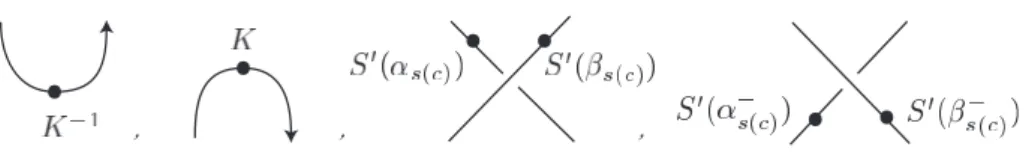
Given a state s∈ S(T), we attach labels on the copies of the fundamental tangles in the diagram following the rule described in Figure 8, where “S⁰” should be replaced with id if the string is oriented downward, and withSotherwise. For example, for a statet∈ S(B), we put

(11)

, , ,

Figure 8: How to place labels on the fundamental tangles

labels on the diagram ofB as in Figure 7 (c), where we setm=t(c1) and n=t(c2) for the upper and the lower crossingsc1andc2, respectively.

We define an element JT ,s ∈ U_h^⊗^ˆⁿ as follows. Theith tensorand ofJT ,s is defined to be the product of the labels put on the component corresponding toTi, where the labels are read off alongT_i reversing the orientation, and written from left to right. We identify the labels S⁰(α^±_i ) and S⁰(β_i^±) with the first and the second tensorands, respectively, of the element S⁰(α^±_i )⊗S⁰(β_i^±)∈U_h^⊗^ˆ². Also we identify the labelK^±¹ with the element K^±¹∈Uh. Then, J_{T ,s} is a well-defined element inU_h^⊗^ˆⁿ. For example, we have

JB,t=S(αm)S(βn)⊗αnβm

=X

q¹²^m(m⁻¹⁾q¹²ⁿ⁽ⁿ⁻¹⁾S(D⁰₁F˜^(m)K⁻^m)S(D₂⁰⁰eⁿ)⊗D⁰₂F˜⁽ⁿ⁾K⁻ⁿD₁⁰⁰e^m

= (−1)^m+nq⁻^n+2mnD⁻²( ˜F^(m)K⁻²ⁿeⁿ⊗F˜⁽ⁿ⁾K⁻^2me^m)∈U_h^⊗^ˆ², whereD=P

D⁰₁⊗D⁰⁰₁ =P

D₂⁰ ⊗D⁰⁰₂.Note thatJT ,s depends on the choice of the diagram.

Set

JT = X

s∈S(T)

JT ,s. For example, we have

JB= X

t∈S(B)

JB,t= X

m,n≥0

(−1)^m+nq⁻^n+2mnD⁻²( ˜F^(m)K⁻²ⁿeⁿ⊗F˜⁽ⁿ⁾K⁻^2me^m).

As is well known [19],JT does not depend on the choice of the diagram, and deﬁnes an isotopy invariant of bottom tangles.

3 Universal invariant of boundary bottom tangles

In this section, we recall Habiro’s formulas for boundary bottom tangles at the topological level (Proposition 3.1), and at the algebraic level on the universal sl2 invariant (Proposition 3.3). Then, we modify these formulas into a form more convenient for our purpose. After that, we study the commutator maps of Uh. In the last section, we give an outline of the proof of Theorem 1.2.

In what follows, we use the following notations. Letη: Q[[h]]→Uhbe the unit morphism ofU_h andµ: U_h^⊗^ˆ²→U_h the multiplication ofU_h. Forg≥0, letµ^[g]: U_h^⊗^ˆ^g→U_hdenote the g-input multiplication deﬁned byµ^[0]=η,µ^[1]= id_U_h,and

µ^[g] =µ^[g⁻^1]◦(µ⊗id^⊗_U^g⁻²

h ), forg≥2.Forg1, . . . , gn≥0, set

µ^[g¹^,...,gⁿ^] =µ^[g¹^]⊗ · · · ⊗µ^[gⁿ^]: U_h^⊗^ˆ^g¹⁺^···^+gⁿ→U_h^⊗^ˆⁿ. (15)

(12)

・・・

・・・・・・

・・・

Figure 9: How to arrange Seifert surfaces

・・・

・・・・・・

・・・

・・・・・・

Figure 10: (a)Y_b^⊗^g(V)∈BTg forV ∈BT2g(b)µ^[g_b¹^,...,gⁿ^](W)∈BTn forW ∈BTg

3.1 Habiro’s formula (topological level)

LetT =T1∪ · · · ∪Tn ∈BTn be a boundary bottom tangle andF1, . . . , Fn mutually disjoint Seifert surfaces such that∂Fi=KT_ifori= 1, . . . , n.We can arrange the surfacesF1, . . . , Fnas depicted in Figure 9, where Double(T⁰) is the tangle obtained from a bottom tangleT⁰∈BT2g, where g = g1+· · ·+gn with gi = genus(Fi), by ﬁrst duplicating and then reversing the orientation of the inner component of each pair of duplicated components.

The above arrangement of the Seifert surfaces implies the following result, which appears in the proof of [4, Theorem 9.9].

Proposition 3.1. For a bottom tangle T ∈BT_n, the following conditions are equivalent.

(1) T is a boundary bottom tangle.

(2) There is a bottom tangle T⁰ ∈ BT2g, g ≥ 0, and integers g1, . . . , gn ≥ 0 satisfying g1+· · ·+gn =g, such that

T =µ_b^[g¹^,...,gⁿ^]Y_b^⊗^g(T⁰), (16) whereY_b^⊗^g: BT_2g→BT_g andµ_b^[g¹^,...,gⁿ^]: BT_g→BT_n are deﬁned as depicted in Figure 10 (a) and (b), respectively.

3.2 Habiro’s formula (algebraic level)

Recall from [4, Proposition 9.7] the commutator morphismYH: H⊗H →Hfor a ribbon Hopf algebraH. In the present case H =Uh, the morphism YU_h: Uh⊗ˆUh→Uhis the continuous Q[[h]]-linear map deﬁned by

YU_h(x⊗y) =X

k≥0

x .

³ βkS¡

(αk. y)(1)

¢´(αk. y)(2)

forx, y∈Uh.

(13)

・・・

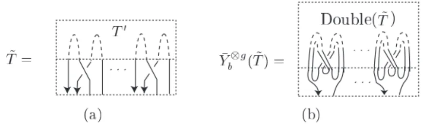
Figure 11: (a) The tangle ˜T =ν_b^⊗^g(T⁰) (b) The bottom tangle ¯Y_b^⊗^g( ˜T)∈BTg

Lemma 3.2 (Habiro [4]). For each bottom tangleT ∈BT_2g,g≥0, we have J_Y⊗g

b (T)=Y_U^⊗^g

h(J_T).

For each bottom tangleT ∈BTg₁+···+g_n,g1, . . . , gn≥0, we have J_µ[g1,...,gn]

b (T)=µ^[g¹^,...,gⁿ^](JT).

Proposition 3.1 and Lemma 3.2 imply the following.

Proposition 3.3 (Habiro [4]). For a boundary bottom tangleT ∈BTn and a bottom tangle T⁰∈BT2g satisfying (16), we have

JT =µ^[g¹^,...,gⁿ^](YU_h)^⊗^g(JT⁰).

3.3 Modiﬁcation of Habiro’s formula (topological level)

In this section, we modify Proposition 3.1.

LetT ∈BTnbe a boundary bottom tangle andT⁰a 2g-component bottom tangle satisfying (16). We decompose the operationY_b^⊗^g into the two operations ν_b^⊗^g and ¯Y_b^⊗^g as follows.

Let ˜T =ν_b^⊗^g(T⁰) be the 2g-component (non-bottom) tangle as depicted in Figure 11 (a). Set Y¯_b^⊗^g( ˜T) =Y_b^⊗^g(T⁰) ∈BT_g, i.e., ¯Y_b^⊗^g( ˜T) is the bottom tangle as depicted in Figure 11 (b), where Double(T⁰) is deﬁned in the same way as that for bottom tangles.

We have

T =µ^[g_b¹^,...,gⁿ^]Y_b^⊗^g(T⁰)

=µ^[g_b¹^,...,gⁿ^]( ¯Y_b^⊗^g◦ν_b^⊗^g)(T⁰)

=µ^[g_b¹^,...,gⁿ^]Y¯_b^⊗^g¡

ν_b^⊗^g(T⁰)¢

=µ^[g_b¹^,...,gⁿ^]Y¯_b^⊗^g( ˜T).

Thus, we can modify Proposition 3.1 by replacing (2) with (2’) as follows.

(2’) There is a 2g-component tangle ˜T = ν_b^⊗^g(T⁰) with T⁰ ∈ BT2g, g ≥ 0, and integers g₁, . . . , g_n≥0 satisfyingg₁+· · ·+g_n=g, such that

T =µ_b^[g¹^,...,gⁿ^]Y¯_b^⊗^g( ˜T).

For a boundary bottom tangle T ∈BTn, we call ( ˜T;g, g1, . . . , gn) as in (2’) a boundary data forT.

(14)

3.4 Modiﬁcation of Habiro’s formula (algebraic level)

Let ¯Y: U_h⊗ˆU_h→U_h be the continuousQ[[h]]-linear map deﬁned by Y¯(x⊗y) =X

x₍₁₎KS(y₍₂₎)KS(x₍₂₎)y₍₁₎, (17) forx, y∈U_h.

We modify Proposition 3.3 as follows.

Proposition 3.4. LetT ∈BT_nbe a boundary bottom tangle and( ˜T;g, g₁, . . . , g_n)a boundary data forT. We have

J_T =µ^[g¹^,...,gⁿ^]Y¯^⊗^g(JT˜).

Here, we can deﬁne the universalsl₂ invariant J_T_˜ ∈U_h^⊗^ˆ^2g of the tangle T˜ in a similar way to that of bottom tangles (cf. [4]).

Letν: Uh⊗Ûh→Uh⊗Ûh be the continuousQ[[h]]-linear map defined by ν(x⊗y) =X

k≥0

xβ_k⊗α_ky, forx, y∈Uh. We reduce Proposition 3.4 to the following lemma.

Lemma 3.5. We have

YU_h = ¯Y ◦ν. (18)

Proof of Proposition 3.4 by assuming Lemma 3.5. LetT⁰∈BTgthe bottom tangle such that T˜ =ν_b^⊗^g(T⁰). We depict in Figure 12 the labels put on the new crossings c1, . . . , cg at the bottom of ˜T associated a states∈ S( ˜T). Since (1⊗S)(R⁻¹) =R, we have