Investigation of Combining Various Major Language Model Technologies including Data Expansion and Adaptation

(1)

PAPER

Special Section on Recent Advances in Machine Learning for Spoken Language Processing

Investigation of Combining Various Major Language Model Technologies including Data Expansion and Adaptation

Ryo MASUMURA^†,††a), Taichi ASAMI^†, Takanobu OBA^†∗, Hirokazu MASATAKI^†, Sumitaka SAKAUCHI^†, andAkinori ITO^††,Members

SUMMARY This paper aims to investigate the performance improvements made possible by combining various major language model (LM) technologies together and to reveal the interactions between LM technologies in spontaneous automatic speech recognition tasks. While it is clear that recent practical LMs have several problems, isolated use of major LM technologies does not appear to offer sufficient performance. In consideration of this fact, combining various LM technologies has been also examined. However, previous works only focused on modeling technologies with limited text resources, and did not consider other important technologies in practical language modeling, i.e., use of external text resources and unsupervised adaptation. This paper, therefore, employs not only manual transcriptions of target speech recognition tasks but also external text resources. In addition, unsupervised LM adaptation based on multi-pass decoding is also added to the combination. We divide LM technologies into three categories and employ key ones including recurrent neural network LMs or discriminative LMs. Our experiments show the effectiveness of combining various LM technologies in not only in-domain tasks, the sub- ject of our previous work, but also out-of-domain tasks. Furthermore, we also reveal the relationships between the technologies in both tasks.

key words: language models, direct decoding, unsupervised adaptation, rescoring, spontaneous speech recognition

1. Introduction

Two statistical models, acoustic models and language models (LMs), are essential components of modern automatic speech recognition systems. This framework was estab- lished many decades ago[1]. Until now, many researchers strove to develop these two statistical models for improving their performance. It can be said that the current progress in speech recognition technology is driven by advancements in these two models.

In recent years, a major breakthrough occurred in acoustic modeling with the introduction of the deep neural network (DNN)[2]. DNNs catch acoustic features more precisely than traditional Gaussian mixture models, and significant performance improvements have been achieved with DNN-based acoustic modeling[3]. Language modeling, however, has seen no comparable breakthrough for a long time even though a lot of LM technologies have been

Manuscript received February 3, 2016.

Manuscript revised May 20, 2016.

Manuscript publicized July 19, 2016.

†The authors are with NTT Media Intelligence Laboratories, NTT Corporation, Yokosuka-shi, 239–0847 Japan.

††The authors are with the Graduate School of Engineering, Tohoku University, Sendai-shi, 980–8579 Japan.

∗Presently, with NTT Docomo Corporation.

a) E-mail: [email protected] DOI: 10.1587/transinf.2016SLP0013

proposed. It is clear that back-offn-gram LMs, the modern practical LMs, have several problems[4]. However, the performance improvements offered by individual LM technologies remain insufficient.

The most likely explanation for the insufficiency is that the problems posed by the back-off n-gram LMs cannot be solved by using just one LM technology. The knowl- edge that individual LM technologies can solve different problems raises the thought that significant performance improvements can be obtained by combining several of them.

This paper identifies the feasibility of this approach and elu- cidates the relationships between LM technologies that are used in concert.

A couple of previous works provide comparative studies of various LM technologies as well as investigations of combining various LM technologies[5]–[7]. The previous works showed that some combinations may theoretically yield much better performance. However, the studies pub- lished to date merely considered the modeling techniques in abstract terms and failed to conduct examinations involving actual speech recognition systems.

In fact, two important issues are raised in the actual use of speech recognition system. The first one is the scarcity of training data. For instance, in the voice search task, it is easy to collect data corresponding to the target task by accessing text-input query logs[8]. In the spontaneous speech task, on the other hand, the data corresponding to the target task must be obtained by manually transcribing speech. Thus, data expansion techniques that can collect useful training data sets from external text resources are important[9]–[12]. In addition, data expansion techniques are useful in addressing the out-of vocabulary (OOV) problem. The second issue is the current weakness of unsupervised adaptation[13]–[15].

Since technologies that offer robust performance in various tasks are difficult to realize, it is important to make LMs that specialize in processing input speech. Unsupervised adaptation is an important approach for realizing these kinds of technologies. We can say that it is necessary to take into account these two issues for our examination since these issues are involved in major problems in back-offn-gram modeling.

This paper, therefore, examines several combinations of various LM technologies, not only modeling technologies but also data expansion and unsupervised adaptation.

This challenge raises, of course, new issues of what kinds of technologies we should use and how to combine diﬀerent Copyright c2016 The Institute of Electronics, Information and Communication Engineers

(2)

kinds of LM technologies. Our contributions to address the issues are summarized as follows.

• We redefine problems posed by traditional back-oﬀn- gram modeling as four items; data sparseness, context limitation, domain dependency, and unawareness of recognition errors.

• We divide LM technologies into three categories (direct decoding, unsupervised adaptation, and rescoring) and prepare the major technologies for each category to totally cover the traditional problems.

• We present combination methods for each category and examine various combination settings to reveal relationships between the technologies.

This paper is an extended study of our previous work[16].

The previous work only examined in in-domain tasks. In this paper, we extend our evaluation to not only in-domain tasks but also out-of-domain tasks.

This paper is organized as follows. Section 2 describes baseline LM technologies and their problems. In Sect. 3, we categorize the LM technologies and identify the major LM technologies in each category. In addition, we also explain how to combine technologies. Section 4 describes our experiments and discusses the relationship between the technologies. Section 5 concludes this paper.

2. Baseline LM Technology and Problems 2.1 Back-OﬀN-gram LMs

The back-off n-gram modeling is the most popular and practical LM[17]. Back-offn-gram LMs are widely used because of their compactness, power, and suitability for ordinary decoder such as weighted finite state transducer (WFST) based decoder[18], [19]. Back-off n-gram LMs calculate the generative probability of wordwkgiven context informationukusingn−1 words behindwk. The generative probability is defined as:

P(wk|uk,Θ1)≈P(wk|wk−n+1, . . . , wk−1,Θ1), (1) wherenis the n-gram order andΘ1is the model parameter.

We note that smoothing techniques are usually used for tackling the zero frequency problem in n-gram modeling[20].

This paper starts with manual transcriptions of a target speech recognition task and develops a baseline system consists of back-oﬀn-gram LMs trained from the transcriptions. A hierarchical Pitman-Yor LM (HPYLM) is used for the back-oﬀn-gram structure[21]. HPYLM is a theoretically elegant Bayesian n-gram model that has demonstrated top performance among several smoothing methods[22].

2.2 Problems

There are obvious problems with back-oﬀ n-gram LMs given the limited availability of manual transcriptions of the target speech recognition task[4]. Fundamental problems can summarized as follows although these problems are not

clearly independent of each other.

• Data sparseness:

If the manual transcriptions of the target speech recognition task are only used for training data, the data size is insufficient to construct robust back-offn-gram LMs to the target tasks. (even though the back-off n-gram LM can assign generative probabilities to linguistic phenomena that are not included in the training data). In addition, OOV words that are not included in the vocabulary have zero probability. For the precise probability estimation, a huge amount of training data is needed.

• Context limitation:

A back-oﬀn-gram LM can consider onlyn−1 words behind the target word. nis usually set to 3-5. Thus, only short context information is used for calculating generative probabilities in back-oﬀn-gram modeling.

It can be expected that long-range context information would yield more precise probability estimation.

• Domain dependency:

The performance of a back-oﬀ n-gram LM depends on the properties of its training data. In fact, an LM constructed using data drawn from many domains is not versatile. It is important to construct domain- dependent LMs to improve LM performance.

• Unawareness of recognition errors:

Back-oﬀ n-gram LMs are usually constructed from text data that does not include mis-recognized words.

Therefore, the concept of recognition error is not considered at all. We can expect performance improvements by explicitly modeling recognition errors.

3. Combinations of Various LM Technologies

3.1 Categorization of LM Technologies

This paper introduces the key kinds of LM technologies. For combining them, it is important to take account of the applicable scope of each technology. In this paper, we consider the following three categories of the situations where a spe- cific LM technology is used.

• Direct decoding:

This category is referred to as back-oﬀ n-gram LM- based methods that can be used in direct (one-pass) decoding. Direct decoding is the ideal form of speech recognition. It basically demands the use of a back- oﬀ n-gram LM suitable for WFST decoders; along this line, we can introduce n-gram approximation techniques or data expansion techniques to tackle the data sparseness problem.

• Unsupervised adaptation:

This category is referred to as back-oﬀ n-gram LM- based methods that require multi-pass decoding for domain adaptation. Unsupervised adaptation can construct LMs dependent on the processing input speech

(3)

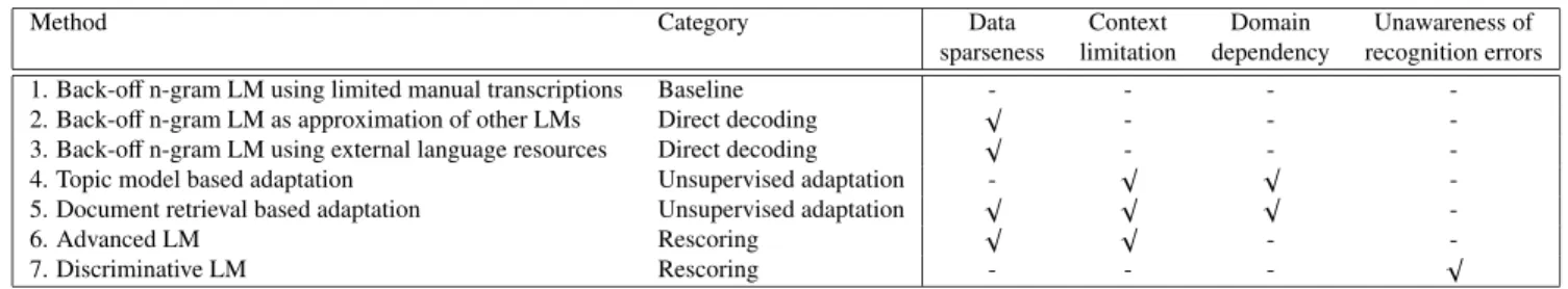
Table 1 Summarization of major LM technologies for each category.

Method Category Data Context Domain Unawareness of

sparseness limitation dependency recognition errors

1. Back-oﬀn-gram LM using limited manual transcriptions Baseline - - - -

2. Back-oﬀn-gram LM as approximation of other LMs Direct decoding √ - - -

3. Back-oﬀn-gram LM using external language resources Direct decoding √

- - -

4. Topic model based adaptation Unsupervised adaptation - √ √ -

5. Document retrieval based adaptation Unsupervised adaptation √ √ √

-

6. Advanced LM Rescoring √ √ - -

7. Discriminative LM Rescoring - - - √

using recognition hypothesis generated in first decoding pass. It can also reflect long-range information through the consideration of overarching recognition hypotheses. The adapted LM is also used in WFST- based decoder.

• Rescoring:

This category is referred to as more complicated model-based methods that cannot be directly introduced to decoding process. Rescoring is performed after recognition hypotheses are obtained, which makes it easy to apply complicated techniques with remarkable properties.

This paper draws several technologies from each category, see Table 1. It is clear that each technology can solve diﬀerent problems posed by back-oﬀn-gram LMs. The details of each technology are given in the following subsec- tions.

3.2 Technologies for Direct Decoding

3.2.1 Back-Oﬀ N-gram LM as Approximation of Other LMs

To construct robust back-offn-gram LMs, we can introduce techniques that convert different kinds of LMs into back-off n-gram structures[23],[24]. In this framework, an LM is constructed from training data for text generation, and texts are then generated by the model via random sampling. Next, a back-offn-gram LM is trained using the generated data.

In this paper, we use latent words LMs (LWLMs) for text generation[23]. LWLMs are generative models, where each latent variable is associated with an observed word[25]. It is expected that the generated data contains various linguistic expressions that are not contained in the original training data. In constructing a back-oﬀn-gram LM from generated data, entropy pruning can be used to reduce the model size[26]. A probability of the resulting back-oﬀ n-gram LM is denoted asP(wk|uk,Θ2).

3.2.2 Back-Oﬀ N-gram LM Using External Text Re- sources

To construct back-oﬀn-gram LM with voluminous training data, we can employ data expansion techniques from external text resources such as Web data[9]–[12].

As the data expansion method, this paper uses the difference in entropy between in-domain and out-of-domain models[12]. In this framework, the in-domain LM is constructed from training data, while the out-of-domain LM is constructed from data randomly extracted from external text resources. The back-oﬀn-gram LM can be also used as each LM.HI(s) is the entropy of sentencesin the in-domain LM, HO(s) is the entropy ofsin the out-of-domain LM; sentence scoreD(s) is defined as:

D(s)=HI(s)−HO(s). (2) We collect sentences whose score is less than threshold T as training data to construct the back-oﬀn-gram LM. In this paper we setT to 0, which is equivalent to using the Bayes classifier for sentence selection[11]. A probability of the resulting back-oﬀn-gram LM is denoted asP(wk|uk,Θ3).

3.2.3 Combination of Technologies for Direct Decoding In direct decoding, each technology generates a back-oﬀn- gram LM as well as a baseline back-oﬀn-gram LM, so we can combine the technologies by using the n-gram mixture model approach. The generative probability is calculated as:

P(wk|uk,Θ1+2+3)=

t∈1,2,3

λtP(wk|uk,Θt), (3)

whereλtis a mixture weight that is preliminarily optimized using a validation set and the EM algorithm. Θ1+2+3 is the model parameter of the n-gram mixture model. The resulting model can be also used in direct decoding since it can be approximated as a single back-oﬀn-gram structure.

3.3 Technologies for Unsupervised Adaptation 3.3.1 Topic Model Based Adaptation

For unsupervised adaptation of back-oﬀn-gram LM, topic models can be used. In unsupervised adaptation with topic models, the entire topic information of the processing target speech is determined by the recognition hypothesis generated in the first pass, and the n-gram model is adapted using the estimated topic. This paper uses the unigram marginal technique since it allows back-oﬀprobabilities in the n-gram model to be considered[27],[28]. We use latent Dirichlet allocation (LDA) as the topic model[29].

(4)

In this framework, the topic probability is estimated using a recognition hypothesis of the target speech, and next, the n-gram model is adapted using the estimated unigram probability. When the baseline model is used in the first pass, adapted n-gram modelP(wk|uk,Θ1+4) is given by:

P(wk|uk,Θ1+4)=

zP(wk|z,Θ4)P(z|d,Θ4) P(wk|Θ1)

_μ

P(wk|uk,Θ1)

Z(uk) , (4) where z is a topic, and d is a recognition hypothesis.

P(wk|z,Θ4) andP(z|d,Θ4) are calculated based on LDA.μ is a tuning parameter andZ(uk) is a normalization term. If P(wk|uk,Θ1+2+3) is used in the first pass, “1” in Eq. (4) is replaced by “1+2+3”.

3.3.2 Document Retrieval Based Adaptation

Relevant documents to a target speech can be utilized for constructing domain-dependent LM. Document retrieval based unsupervised adaptation can be split into the following steps. First, relevant data is selected from external text resources using a recognition hypothesis of the target speech. Next, the back-oﬀ n-gram model is adapted using relevant documents[13],[14],[30],[31]. Various methods have been proposed for document retrieval. One study uses several document retrieval techniques[32]. In this paper, we use vector space models (VSMs) for document retrieval[13],[14],[30].

Document retrieval based on VSMs uses the cosine similarity between the recognition hypothesis and a text in the external resources. After retrieval, unsupervised adaptation is conducted by mixing the baseline n-gram model with the n-gram model constructed from the relevant documents.

When the baseline model is used in the first pass, adapted n-gram modelP(wk|uk,Θ1+5) is given by:

P(wk|uk,Θ1+5)=

λ5P(wk|uk,Θ1)+(1−λ5)P(wk|uk,Θ5), (5) where P(wk|uk,Θ5) is the back-oﬀ n-gram model constructed from relevant documents. λ5 is a mixture weight that is automatically optimized using the recognition hypothesis[33]. If P(wk|uk,Θ1+2+3) is used in the first pass,

“1” in Eq. (5) is replaced by “1+2+3”.

3.3.3 Combination of Technologies for Unsupervised Adaptation

In unsupervised adaptation, adapted models based on each technique are expressed as n-gram models, so we can also combine the techniques as n-gram mixture models. The adapted n-gram model that uses both unsupervised adaptation technologies is expressed as:

P(wk|uk,Θ1+4+5)=

λaP(wk|uk,Θ1+4)+(1−λa)P(wk|uk,Θ1+5), (6)

where Θ1+4+5 is the model parameter. In contrast to direct decoding, mixture weight λa is optimized using the recognition hypothesis generated in the first pass. Also, if P(wk|uk,Θ1+2+3) is used in the first pass, “1” in Eq. (6) is replaced by “1+2+3”.

3.4 Technologies for Rescoring 3.4.1 Advanced LMs

Beyond the back-oﬀn-gram structure, various model structures such as neural networks and random forests have been proposed[34], [35]. Of particular interest, recurrent neural network LMs (RNNLMs) have attracted significant at- tention in recent years[36]. RNNLMs have two characteristics: one is that the word space can be represented as a continuous space vector based on neural networks, and the other is that long-range information can be flexibly taken into consideration based on its recurrent structure. Since using an RNN makes the cost of computing the probability estimation proportional to the lexical size of the output layer, class-based RNNLMs are most commonly used[37].

The resulting probability estimation is defined as:

P(wk|uk,Θ6)=P(wk|sk,ck,Θ6)P(ck|sk,Θ6), (7) where s is context information, which includes the previous word and previous output in the hidden layer, and cis word class. Θ6 denotes the model parameter of RNNLM.

In rescoring, we use the probability obtained by linearly in- terpolating RNNLM and the back-oﬀn-gram model that is employed in the decoding part. When the baseline model is used in the decoding part, the mixed probability is given by:

P(wk|uk,Θ1+6)=

λ6P(wk|uk,Θ1)+(1−λ6)P(wk|uk,Θ6), (8) where λ6 is a mixture weight which is preliminarily defined by processing the validation set. If the adapted model P(wk|uk,Θ1+2+3+4+5) is used in decoding part, “1” in Eq. (8) is replaced by “1+2+3+4+5”.

3.4.2 Discriminative LMs

Discriminative LMs (DLMs) are constructed from pairs of reference and error words while standard LMs consider correct word sequences. DLMs, also called error corrective models or re-ranking models, can evaluate whether a recognition hypothesis is correct or incorrect[38]. The n- best list generated from a speech recognizer is denoted as L={dj|j=1,· · ·,m}wheredjis the j-th hypothesis in the n-best list. Error correction using a DLM is realized as:

d^∗=arg max

d∈L

{a0f0(d)+af(d)}, (9) where f(d) is the feature vector ofdand f0(d) is the speech recognition score ofd.a0andadenote a scaling factor and model parameter of DLM, respectively. The scaling factor is

(5)

preliminarily defined by processing the validation set. There are several methods to estimate the model parameter[39].

We use round-robin duel discrimination (R2D2) for this estimation[40]as it outperforms other methods under many conditions.

3.4.3 Combination of Technologies for Rescoring In rescoring, RNNLM has a diﬀerent structure from DLM, so the techniques are introduced in sequence. In fact, DLM must be introduced at the end because it is used for error correction. Therefore, RNNLM-based rescoring is conducted first based on the mixed score yielded by back-oﬀn- gram LM and RNNLM. After adding RNNLM, DLM-based rescoring is conducted. In this case, the speech recognition score contains the RNNLM-based score.

4. Experiments

4.1 Setups

Our experiments used the Corpus of Spontaneous Japanese (CSJ)[41]. CSJ was divided into a training set (Train), training set for DLM (Train DLM), validation set (Valid), and test set A (Test A) and B (Test B). The validation set was used for optimizing several hyper parameters. In addition, we also employed the Corpus of spoken Japanese Lecture Contents (CJLC) as test set C (Test C) for evaluations in out-of-domain environments[42]. Details of the data sets are shown in Table 2.

We also prepared text data of about 50 billion morphemes drawn from the web as the external text resource.

We used an acoustic model based on hidden Markov models with DNN (DNN-HMM)[2],[3]. The trained DNN-HMM had 8 hidden layers with 2048 nodes and 3072 outputs. The speech recognition decoder was VoiceRex, a WFST-based decoder[19],[43]. JTAG was used as the morpheme analyzer to split sentences into words[44].

Our evaluation examined the following methods.

These methods and the numbers correspond to Table 1 en- tries. We combined these methods category-wise and then all of them.

1. Back-oﬀ n-gram LM using limited manual tran- scriptions: word-based 3-gram HPYLM constructed from the training set. For the training, we used 200 iterations for burn-in, and collected 10 samples. No pruning technique was used. Vocabulary size was 78K words.

Table 2 Experimental data set.

Domain # of documents # of morphemes

Train CSJ 2,472 6,752,588

Train DLM CSJ 200 542,215

Valid CSJ 10 28,547

Test A CSJ 10 28,504

Test B CSJ 10 18,426

Test C CJLC 6 53,828

2. Back-oﬀ n-gram LM as approximation of other LMs:word-based 3-gram HPYLM constructed from 1 billion morphemes generated based on LWLM. LWLM was constructed from the training set. For the training of HPYLM, we used 200 iterations for burn-in, and collected 10 samples. Entropy based pruning was conducted to reduce the model size. Vocabulary size was 78K words, which corresponds to the baseline.

3. Back-oﬀ n-gram LM using external language re- sources: word-based 3-gram HPYLM constructed from 2 billion morphemes selected from the external text resources. For the training of HPYLM, we used 200 iterations for burn-in, and collected 10 samples.

Entropy based pruning was used. As a limited vocabulary setup, we used vocabulary consisted of 78K words, which corresponds to the baseline. As an expanded vocabulary setup, we selected top 600K words based on word frequency. The expanded vocabulary setup is denoted as 3.

4. Topic model based adaptation:unsupervised adaptation using the unigram marginal technique and LDA.

LDA was constructed from a training set containing 50 topics. Tuning parameter was set to 0.5. The vocabulary size of the adapted model was 78K.

5. Document retrieval based adaptation:unsupervised adaptation based on document retrieval using a vector space model. We selected top 1K documents from external text resources and constructed word-based 3- gram HPYLM from them. As a limited vocabulary setup, the vocabulary size of the adapted model was restricted to 78K, which corresponds to the baseline.

Moreover, a vocabulary-limitation-free model, which uses all of words in retrieved documents for the domain adaptation, was also prepared as an expanded vocabulary setup 5. Note that the vocabulary size is not constant because retrieved documents are diﬀerent ac- cording to target speech.

6. Advanced LM: class-based RNNLM constructed from the training set. It used 500 hidden neurons, 1000 classes. Vocabulary size was 78K words, which corresponds to the baseline.

7. Discriminative LM: DLM with word features constructed from training data for DLM. R2D2 method was used for training. To generate recognition hypotheses about the training data, we used two kinds of models. One is the baseline system and the other is a system that combined all techniques except DLM. The latter is denoted as 7^∗.

Note that the expanded vocabulary setups (3 and 5) can be conducted when external text resources were used. Also, setups that combined 3or 5with other methods mean the expanded vocabulary setups. When we used the methods for rescoring (6 and 7), we generated 1000-best lists in decoding part. Several hyper parameters for each method and the

(6)

Table 3 Experimental results on validation set: PPL, WER [%], OOV rate [%], and RTF.(a)-(q) are limited vocabulary setups and(r)-(z)are expanded vocabulary setups. No PPL comparison is possible among setups with diﬀerent vocabulary size.

Setup Mixture weights Vocabulary Number of Valid

(optimized using validation set) size parameters (CSJ)

PPL WER OOV rate RTF

Limited vocabulary setups

(a) 1. - 78K 26M 83.18 20.01 0.73 0.75

(b) 2. - 78K 80M 85.45 20.15 0.73 0.77

(c) 1+2. λ1=0.53, λ2=0.47 78K 103M 77.86 19.16 0.73 0.85

(d) 3. - 78K 254M 140.86 22.95 0.73 0.90

(e) 1+3. λ¹=0.77, λ³=0.23 78K 272M 77.77 18.84 0.73 0.92

(f) 1+2+3. λ1=0.47, λ2=0.35, λ3=0.18 78K 320M 74.89 18.45 0.73 0.90

(g) 1+4. - 78K 31M 71.87 19.29 0.73 1.45

(h) 1+5. - 78K 88M 71.47 18.38 0.73 5.66

(i) 1+4+5. - 78K 92M 65.24 18.07 0.73 5.74

(j) 6. - 78K 780M 77.50 - 0.73 -

(k) 1+6. λ6=0.42 78K 806M 71.70 19.01 0.73 1.28

(l) 1+7. 78K 33M - 19.28 0.73 0.79

(m) (1+6)+7. - 78K 813M - 18.25 0.73 1.32

(n) (1+2+3)+4+5. - 78K 365M 64.53 17.49 0.73 6.14

(o) (1+2+3+4+5)+6. λ6=0.64 78K 1145M 61.32 17.23 0.73 6.57

(p) (1+2+3+4+5+6)+7. - 78K 1152M - 16.51 0.73 6.61

(q) (1+2+3+4+5+6)+7^∗. - 78K 1152M - 16.45 0.73 6.61

Expanded vocabulary setups

(r) 3. - 600K 340M 149.79 22.95 0.37 1.01

(s) 1+3. λ1=0.74, λ3=0.26 657K 355M 83.98 18.45 0.05 1.02

(t) 1+2+3. λ1=0.45, λ2=0.34, λ3=0.21 657K 410M 81.12 18.12 0.05 1.04

(u) 1+5. - 254K 113M 75.45 18.26 0.13 6.81

(v) 1+4+5. - 254K 117M 69.01 17.88 0.13 6.90

(w) (1+2+3)+4+5. - 688K 470M 69.93 17.26 0.05 7.48

(x) (1+2+3+4+5)+6. λ6=0.67 688K 1250M 67.32 17.08 0.05 8.01

(y) (1+2+3+4+5+6)+7. - 688K 1254M - 16.25 0.05 8.05

(z) (1+2+3+4+5+6)+7^∗. - 688K 1254M - 16.20 0.05 8.05

combined methods were optimized using validation set.

4.2 Results

Table 3 and Table 4 show the perplexity (PPL), word error rate (WER), and OOV rate results for each setup in validation set and test sets. We labeled the experimental conditions from(a)to (z)where each number corresponds to our experimental setup and Table 1. We evaluated both limited vocabulary setups (a)-(q)and expanded vocabulary setups(r)-(z). No PPL comparison is possible for the expanded vocabulary setups as they have diﬀerent vocabulary sizes from the baseline vocabulary. In addition, Table 3 shows real time factor (RTF) results which include not only decoding time but also adaptation and rescoring time for the validation set. Also, Table 3 displays number of parameters and mixture weights (λ1, λ2, λ3, λ6) that were preliminarily optimized using the validation set. Note that other mixture weights (λ5, λa) are dynamically determined by a recognition hypothesis of a target speech. There are no WER results in(j)since RNNLM cannot be applied to ASR directly.

On the other hand, there are no PPL results in introducing DLM,(l),(m),(p),(q),(y),(z), because DLM is not a probabilistic model.

Task diﬃculties can be shown in Table 3 and Table 4.

They show that test set C was more diﬃcult than the validation set and test sets A and B. WER in Test C was about 40

% while WER in the others was about 20 %. This is because test set C is a diﬀerent domain from that of the training data.

First, we evaluated RTF results and number of parameters of each setup. From the viewpoint of RTF, direct decoding methods such as(c)or(e)had time eﬃciency compared to the other setups. Unsupervised adaptation methods such as(g)or(h)took much time because they conducted LM adaptation and second pass decoding. In rescoring methods, DLM took less time than RNNLM. From the viewpoint of number of parameters, RNNLM required much more parameters than other conditions. Also, use of external text resources increased number of parameters. In comparison to the baseline(a), RTF was increased to about 11-fold, and number of parameters was increased to about 48-fold when we used all of LM technologies(z).

Next, we evaluated the performance of combining various LM technologies under the constraint of limited vocabulary setups (a)-(q). We could achieve performance improvements by combining technologies compared to the baseline (a). For instance, (c)and (e)are more eﬀec- tive than(a). Moreover, we could obtain further improvements by combining LM technologies in each category compared to using only a single technique in each category. For instance, (f)is more eﬀective than (c)or (e). This result shows that individual technologies in each category can complement each other. The best performance was obtained when all technologies were combined and matched DLM

(7)

Table 4 Experimental results on test sets: PPL, WER [%], and OOV rate [%]. (a)-(z)are corresponds to Table 3. Test A and Test B are in-domain tasks, and Test C is out-of-domain task. No PPL comparison is possible among setups with diﬀerent vocabulary size.

Setup Test A Test B Test C

(CSJ) (CSJ) (CJLC)

PPL WER OOV rate PPL WER OOV rate PPL WER OOV rate

Limited vocabulary setups

(a) 1. 70.72 24.46 0.54 102.44 23.03 1.08 169.03 43.97 3.67

(b) 2. 74.36 24.58 0.54 107.16 22.94 1.08 149.61 43.12 3.67

(c) 1+2. 67.42 23.49 0.54 96.79 22.27 1.08 143.78 42.40 3.67

(d) 3. 135.34 27.90 0.54 129.15 23.46 1.08 179.81 46.27 3.67

(e) 1+3. 67.09 23.04 0.54 88.91 21.06 1.08 132.21 42.37 3.67

(f) 1+2+3. 64.92 22.70 0.54 87.43 20.80 1.08 126.93 42.11 3.67

(g) 1+4. 64.87 23.80 0.54 95.12 22.66 1.08 162.95 43.50 3.67

(h) 1+5. 64.82 22.74 0.54 87.37 21.23 1.08 154.07 42.19 3.67

(i) 1+4+5. 60.60 22.61 0.54 82.82 21.03 1.08 149.33 42.00 3.67

(j) 6. 68.10 - 0.54 98.23 - 1.08 172.48 - 3.67

(k) 1+6. 63.29 23.34 0.54 93.96 22.05 1.08 151.13 43.41 3.67

(l) 1+7. - 23.22 0.54 - 21.96 1.08 - 42.91 3.67

(m) (1+6)+7. - 22.32 0.54 - 20.92 1.08 - 42.61 3.67

(n) (1+2+3)+4+5. 59.89 21.56 0.54 81.69 20.12 1.08 122.78 41.37 3.67

(o) (1+2+3+4+5)+6. 56.74 21.34 0.54 77.56 19.96 1.08 119.32 41.34 3.67

(p) (1+2+3+4+5+6)+7. - 20.47 0.54 - 18.84 1.08 - 40.54 3.67

(q) (1+2+3+4+5+6)+7^∗. - 20.38 0.54 - 18.70 1.08 - 40.33 3.67

Expanded vocabulary setups

(r) 3. 141.39 28.38 0.57 141.45 22.75 0.48 211.61 45.66 0.72

(s) 1+3. 70.17 22.45 0.10 99.43 19.71 0.07 168.72 41.85 0.19

(t) 1+2+3. 68.58 21.96 0.10 97.35 19.34 0.07 159.81 41.36 0.19

(u) 1+5. 67.26 22.62 0.18 99.94 20.03 0.13 176.12 41.36 0.53

(v) 1+4+5. 63.97 22.45 0.09 90.11 19.89 0.03 173.06 41.06 0.18

(w) (1+2+3)+4+5. 62.85 21.44 0.09 91.57 18.91 0.03 155.53 40.51 0.18 (x) (1+2+3+4+5)+6. 60.62 21.27 0.09 89.14 18.75 0.03 152.42 40.45 0.18

(y) (1+2+3+4+5+6)+7. - 20.32 0.09 - 17.95 0.03 - 39.78 0.18

(z) (1+2+3+4+5+6)+7^∗. - 20.17 0.09 - 17.92 0.03 - 39.66 0.18

was used. In terms of WER, statistically significant performance improvements (p <0.001) were achieved by(n) compared to the baseline(a)in each test set.

In addition, we evaluated the expanded vocabulary setups(r)-(z). Tables 3 and 4 show that the vocabulary expansion can improve OOV rate compared to the limited vocabulary setups. In direct decoding, the WER differences between(f)and(t)in each test sets were statistically significant (p <0.05). Also, in unsupervised adaptation, the WER differences between(i)and(v)in test sets B and C were statistically significant (p <0.01) although the WER difference in test set A was no statistically significant (p >

0.05). It seems that these improvements were induced by OOV rate improvements. In test set A, OOV rate of the baseline vocabulary was comparatively small, so vocabulary expansion was not so eﬀective. The highest performance was attained by(z) that combined all techniques with vocabulary expansion. In terms of WER, it yielded 4-5 point error reduction compared to the baseline(a)in each test sets. The improvements were statistically significant (p <0.001). These results suggested that remarkable performance improvements are possible by simultaneously tackling multiple LM problems.

4.3 Discussions

We discuss relationships between the technologies. Four

Table 5 First notable point in experimental results: WER [%] and RER [%]. The RER results with a dagger^†are statistically significant (p<0.01).

Test A Test B Test C

(CSJ) (CSJ) (CJLC)

WER RER WER RER WER RER

(a) 24.46 - 23.03 - 43.97 -

→(c) 23.49 ^†3.96 22.27 3.30 42.40 ^†3.57

→(s) 22.45 ^†8.21 19.71 ^†14.45 41.85 ^†4.82

→(t) 21.96 ^†10.22 19.34 ^†16.02 41.36 ^†5.93

notable points can be extracted from Tables 3 and 4.

First, Table 5 summarized the WER and relative error reduction (RER) results to reveal characteristics of direct decoding based on n-gram modeling. The result shows that building a back-offn-gram LM with combining technologies for direct decoding showed substantial performance improvements. The WER differences between (a)and(t) were statistically significant (p <0.01) in each test set. In particular, (s)was effective for test set B. This is because OOV words were decreased by using external text resources.

These results show that significant performance improvements are possible by solving a data sparseness problem even if the model structure is a back-oﬀn-gram LM.

Second, Table 6 summarizes the WER and RER results to reveal characteristics of unsupervised adaptation for back-oﬀn-gram modeling. The result shows that there was only a slight improvement in performing unsupervised

(8)

Table 6 Second notable point in experimental results: WER [%] and RER [%]. The RER results with a dagger^† are statistically significant (p<0.01).

(CSJ) (CSJ) (CJLC)

(a) 24.46 - 23.03 - 43.97 -

→(v) 22.45 ^†8.21 19.89 ^†13.63 41.06 ^†6.61

(t) 21.96 - 19.34 - 41.36 -

→(w) 21.44 2.36 18.91 2.22 40.51 ^†2.05

Table 7 Third notable point in experimental results: WER [%] and RER [%]. The RER results with a dagger^† and an asterisk^∗are statistically significant (p<0.01 andp<0.05, respectively).

(CSJ) (CSJ) (CJLC)

(a) 24.46 - 23.03 - 43.97 -

→(k) 23.34 ^†4.57 22.05 ^∗4.25 43.41 1.27

(w) 21.44 - 18.91 - 40.51 -

→(x) 21.27 0.79 18.75 0.85 40.45 0.15

adaptation after constructing the back-offn-gram LM with combining technologies for direct decoding for in-domain tasks. In test sets A and B, the WER differences between (t) and(w) were no statistically significant (p > 0.05) while the WER differences between(a)and(v)were statistically significant (p<0.01). Even if we use the technologies for direct decoding, a context limitation problem cannot be solved. This result shows that using long-range information offers comparatively small benefit. On the other hand, unsupervised adaptation was significantly effective (p <

0.01) for our-of-domain task even if we use LM with technologies for direct decoding. This is because the back-oﬀ n-gram LM used in the first pass did not well match the test set C. It suggests that LM adaptation is necessary to solve a domain dependency problem.

Third, Table 7 summarizes the WER and RER results to reveal relationships between RNNLM and back-off n- gram modeling. The result shows that the improvements offered by RNNLM were small after performing technologies for direct decoding and unsupervised adaptation. In test sets A and B, the WER differences between (w)and (x)were no statistically significant (p >0.05) while the WER differences between(a) and(k) were statistically significant (p <0.05). While it can be expected to solve a data sparseness problem and a context limitation problem by introducing RNNLM, it suggests that back-offn-gram LM can offer similar effect by raising the robustness through the use of technologies for direct decoding and by reflecting the long-range information based on unsupervised adaptation.

In addition, RNNLM was comparatively ineﬀective for out- of-domain task. There was no statistically significance (p>

0.05) between(a)and(k)in test set C. The main reason is that RNNLM is weak against the domain dependency problem as is standard back-oﬀn-gram modeling.

Fourth, Table 8 summarizes the WER and RER results to reveal relationships between DLM and other

Table 8 Fourth notable point in experimental results: WER [%] and RER [%]. The RER results with a dagger^† and an asterisk^∗ are statistically significant (p<0.01 andp<0.05, respectively).

(CSJ) (CSJ) (CJLC)

(a) 24.46 - 23.03 - 43.97 -

→(l) 23.22 ^†5.06 21.96 ^∗4.64 42.91 ^†2.41

(x) 21.27 - 18.75 - 40.45 -

→(y) 20.32 ^†4.46 17.95 ^∗4.26 39.78 ^∗1.65

→(z) 20.17 ^†5.17 17.92 ^∗4.42 39.66 ^†1.95

technologies. The result shows that DLM always demonstrated a fixed improvement even if used at the end. In fact, the WER differences between(a)and(l), and those between (x)and (y)or (z)were individually statistically significant (p<0.05) in each test set. This attributed to the fact that DLMs have a different aspect from other modeling techniques. It is clear that the input may not fully resolved if only correct word sequences are modeled, so the framework of modeling the speech recognition error directly is an effective solution. On the other hand, the WER differences between(y)to(z)were statistically no significant (p>0.05) even though DLM was trained using the recognition hypothesis generated from a matched system. It can be also considered that recognition errors that can be improved by DLMs have similar patterns between the baseline system and the matched system. Also, DLM was effective for not only in-domain tasks but also out-of-domain tasks. It can be considered that DLMs with R2D2 method can perform robustly with multiple domains.

5. Conclusions

In this paper, we examined the combination of various LM technologies including data expansion via external language resources and unsupervised adaptation in the spontaneous speech recognition task. To this end, We redefined problems posed by traditional back-oﬀ n-gram modeling and employed the major LM technologies with consideration of their applicable scope in the actual use of speech recognition system. We demonstrated that significant performance improvements were possible by combining various technologies, compared to using each technology in isolation. Com- bining all technologies yielded 4-5 point error reduction in WER. Furthermore, our investigation revealed several remarkable facts: the power of a back-oﬀn-gram modeling with combining technologies for direct decoding including vocabulary expansion, the relationship between RNNLM rescoring or unsupervised adaptation and other technologies, and the uniqueness of DLM.

References

[1] S. Young, “A review of large-vocabulary continuous-speech recognition,” IEEE Signal Process. Mag., vol.13, pp.45–57, 1996.

[2] G. Hinton, L. Deng, D. Yu, G. Dahl, A. rahman Mohamed, N. Jaitly, A. Senior, V. Vanhoucke, P. Nguyen, T. Sainath, and B. Kingsbury,

(9)

“Deep neural networks for acoustic modeling in speech recognition,” IEEE Signal Processing Magazine, vol.29, pp.82–97, 2012.

[3] F. Seide, G. Li, and D. Yu, “Conversational speech transcription using context-dependent deep neural networks,” In Proc. INTER- SPEECH, pp.437–440, 2011.

[4] R. Rosenfeld, “Two decades of statistical language modeling: Where do we go from here?,” Proc. IEEE, vol.88, no.8, pp.1270–1278, 2000.

[5] S.F. Chen and J. Goodman, “An empirical study of smoothing techniques for language modeling,” Computer Speech & Language, vol.13, no.4, pp.359–393, 1999.

[6] T. Mikolov, A. Deoras, S. Kombrink, L. Burget, and J. Cernocky,

“Empirical evaluation and combination of advanced language modeling techniques,” In Proc. INTERSPEECH, pp.605–608, 2011.

[7] C. Chelba, T. Mikolov, M. Schuster, Q. Ge, T. Brants, P. Koehn, and T. Robinson, “One billion word benchmark for measur- ing progress in statistical language modeling,” In Proc. INTER- SPEECH, pp.2635–2639, 2014.

[8] C. Chelba, J. Schalkwyk, T. Brants, V. Ha, B. Harb, W. Neveitt, C.

Parada, and P. Xu, “Query language modeling for voice search,” In Proc. SLT, pp.127–132, 2010.

[9] D. Klakow, “Selecting articles from the language model training corpus,” In Proc. ICASSP, vol.3, pp.1695–1698, 2000.

[10] I. Bulyko, M. Ostendorf, M. Siu, T. Ng, A. Stolcke, and ¨O. C¸ etin,

“Web resources for language modeling in conversational speech recognition,” ACM Transactions on Speech and Language Process- ing, vol.5, no.1, pp.1–25, 2007.

[11] R. Masumura, S. Hahm, and A. Ito, “Training a language model using webdata for large vocabulary Japanese spontaneous speech recognition,” In Proc. Interspeech 2011, pp.1465–1468, 2011.

[12] R.C. Moore and W. Lewis, “Intelligent selection of language model training data,” In Proc. ACL, pp.220–224, 2010.

[13] L. Chen, J.L.G.L. Lamel, G. Adda, and M. Adda, “Using information retrieval methods for language model adaptation,” In Proc.

EUROSPEECH, pp.255–258, 2001.

[14] T. Niesler and D. Willet, “Unsupervised language model adaptation for lecture speech transcription,” In Proc. ICSLP, pp.1413–1416, 2002.

[15] M. Bacchiani and B. Roark, “Unsupervised language model adaptation,” In Proc. ICASSP, pp.224–227, 2003.

[16] R. Masumura, T. Asami, T. Oba, H. Masataki, S. Sakauchi, and A.

Ito, “Combinations of various language model technologies including data expansion and adaptation in spointaneous speech recognition,” In Proc. INTERSPEECH, pp.463–467, 2015.

[17] J.T. Goodman, “A bit of progress in language modeling,” Computer Speech & Language, vol.15, no.4, pp.403–434, 2001.

[18] M. Mohri, F. Pereira, and M. Riley, “Weighted finite-state transduc- ers in speech recognition,” Computer Speech & Language, vol.16, no.1, pp.69–88, 2002.

[19] T. Hori, C. Hori, Y. Minami, and A. Nakamura, “Eﬃcient WFST-based one-pass decoding with on-the-fly hypothesis rescoring in extremely large vocabulary continuous speech recognition,”

IEEE Trans. Audio, Speech, Language Process., vol.15, no.4, pp.1352–1365, 2007.

[20] R. Kneser and H. Ney, “Improved backing-oﬀfor m-gram language modeling,” In Proc. ICASSP, vol.1, pp.181–184, 1995.

[21] Y.W. Teh, “A hierarchical Bayesian language model based on Pitman-Yor processes,” In Proc. COLING/ACL, pp.985–992, 2006.

[22] S. Huang and M. Yor, “Hierarchical Pitman-Yor language models for ASR in meetings,” In Proc. ASRU, pp.124–129, 2007.

[23] R. Masumura, H. Masataki, T. Oba, O. Yoshioka, and S. Takahashi,

“Use of latent words language models in ASR: a sampling-based implementation,” In Proc. ICASSP, pp.8445–8449, 2013.

[24] A. Deoras, T. Mikolov, S. Kombrink, M. Karafiat, and S.

Khudanpur, “Variational approximation of long-span language models in LVCSR,” In Proc. ICASSP, pp.5532–5535, 2011.

[25] K. Deschacht, J.D. Belder, and M.F. Moens, “The latent words

language model,” Computer Speech & Language, vol.26, no.5, pp.384–409, 2012.

[26] A. Stolcke, “Entropy-based pruning of backoﬀlanguage models,”

In Proc. DARPA Broadcast News Transcription and Understanding Workshop, pp.270–274, 1998.

[27] M. Federico, “Language model adaptation through topic decompo- sition and MDI estimation,” In Proc. ICASSP, vol.1, pp.703–706, 2002.

[28] Y.C. Tam and T. Schultz, “Unsupervised language model adaptation using latent semantic marginals,” In Proc. INTERSPEECH, pp.2207–2209, 2006.

[29] D.M. Blei, A.Y. Ng, and M.I. Jordan, “Latent Dirichlet allocation,”

J. Mach. Learn. Res., pp.993–1022, 2003.

[30] R. Masumura, A. Ito, Y. Uno, M. Ito, and S. Makino, “Document expansion using relevant web documents for spoken document retrieval,” In Proc. NLP-KE, pp.612–619, 2010.

[31] R. Masumura, S. Hahm, and A. Ito, “Language model expansion using webdata for spoken document retrieval,” In Proc.

INTERSPEECH, pp.2133–2136, 2011.

[32] H. Nanjo and T. Kawahara, “Language model and speaking rate adaptation for spontaneous presentation speech recognition,”

IEEE Transaction on Speech and Audio Processing, vol.12, no.4, pp.391–400, 2004.

[33] F. Jelinek and R.L. Mercer, “Interpolated estimation of Markov source parameters from sparse data,” pattern Recognition in Prac- tice, pp.381–397, 1980.

[34] Y. Bengio, R. Ducharme, P. Vincent, and C. Jauvin, “A neural probabilistic language model,” J. Mach. Learn. Res., vol.3, pp.1137–1155, 2003.

[35] P. Xu and F. Jelinek, “Random forests in language modeling,” In Proc. EMNLP, pp.325–332, 2004.

[36] T. Mikolov, M. Karafiat, L. Burget, J. Cernocky, and S. Khudanpur,

“Recurrent neural network based language model,” In Proc.

INTERSPEECH, pp.1045–1048, 2010.

[37] T. Mikolov, S.K. Stefan, L. Burget, J. Cernocky, and S. Khudanpur,

“Extensions of recurrent neural network language model,” In Proc.

ICASSP, pp.5528–5531, 2011.

[38] B. Roark, M. Saraclar, and M. Collins, “Corrective language modeling for large vocabulary ASR with the perceptron algorithm,” In Proc. ICASSP, pp.749–752, 2004.

[39] T. Oba, T. Hori, and A. Nakamura, “A comparative study on methods of weighted language model training for reranking LVCSR n-best hypotheses,” In Proc. ICASSP, pp.5126–5129, 2010.

[40] T. Oba, T. Hori, A. Nakamura, and A. Ito, “Round-robin duel discriminative language model,” IEEE Trans. Audio, Speech, Language Process., vol.20, no.4, pp.1244–1255, 2012.

[41] K. Maekawa, H. Koiso, S. Furui, and H. Isahara, “Spontaneous speech corpus of Japanese,” In Proc. LREC, pp.947–952, 2000.

[42] S. Kogure, H. Nishizaki, M. Tsuchiya, K. Yamamoto, S. Togashi, and S. Nakagawa, “Speech recognition performance of CJLC:

Corpus of Japanese lecture contents,” In Proc. INTERSPEECH, pp.1554–1557, 2008.

[43] H. Masataki, D. Shibata, Y. Nakazawa, S. Kobashikawa, A. Ogawa, and K. Ohtsuki, “VoiceRex spontaneous speech recognition technology for contact-center conversations,” NTT Technical Review, vol.5, no.1, pp.22–27, 2007.

[44] T. Fuchi and S. Takagi, “Japanese morphological analyzer using word co-occurrence: JTAG,” In Proc. COLING/ACL, pp.409–413, 1998.