Estimating Discrete-Time Periodic Software Rejuvenation Schedules under Cost Effectiveness Criterion (Mathematics of Decision-making under uncertainty)

Estimating

Discrete-Time Periodic Software

Rejuvenation

Schedules under

Cost Effectiveness Criterion

岩本 一樹\dagger, 土肥 正\dagger, 海生 亘人\ddagger

K. Iwamoto\dagger_{, T. Dohi}\dagger _{and N. Kaio}\ddagger

\dagger _{広島大学大学院工学研究科情報工学専攻}

\ddagger _{広島修道大学経済科学部経営情報学科}

\dagger Graduate_{School of Engineering, Hiroshima University, Japan}

\ddagger_{Facu1ty of Economic Sciences, Hiroshima Shudo University, Japan}

1.

INTRODUCTION

Software faults should ideally have been removed during the debugging phase. Even if software may have been thoroughly tested, it still may have

some

design faults that

are

yet to be revealed. Such faults are called bohrbugs and may exist

even

in mature software

such as commercial operating systems. Also,

even

mature software

can

be expected to

have what areknown as heisenbugs[11]. These

are

bugs in the software thatare revealed only duringspecific collusions of events. For example, asequenceofoperationsmay leave the software in astate that results in an

error on

an operation executed next. Simply retrying afailed operation,orif the applicationprocess hascrashed, restarting the process

might resolve the problem. Another tyPe of fault observed in software systems is due to

the phenomenon of

resource

exhaustion. Operating system

resources

such

as

swap space and free memory available

are

progressively depleted due to defects in software such

as

memory leaks and incomplete cleanup of

resources

after

use.

These faults may exist in the operating system, middleware and the application software.

In fact, when software application executes continuously for longperiodsof time,

some

of the faults

cause

software toagedueto the

error

conditions that

accrue

with time$\mathrm{a}\mathrm{n}\mathrm{d}/\mathrm{o}\mathrm{r}$

load.

_Software

aging will affect the performanceof the application and eventually

cause

it to fail [1, 4, 8, 16]. _{Software aging has also been observed in widely-used software like} Internet Explorer, Netscape and xrn

as

well as commercial operating systems and

mid-dleware. Acomplementary approach to handle software aging and its related transient

software failures, called

_software

rejuvenation, are becoming popular [12]. Software reju-venation isapreventiveand proactivesolution that is particularly useful for counteracting

thephenomenon of software aging. Itinvolves stopping the running software occasionally,

cleaning its internal state and restarting it. Cleaning the internal state of asoftware might involve garbage collection, flushing operating system kernel tables, reinitializing internal data structures, and hardware reboot.

Huang et al. [12] report the software aging phenomenon in real telecommunications

billing application where over time the application experiences acrash or ahang failure,

and propose to perform rejuvenation occasionally or periodically. More specifically, they

consider the degradation as atwo stepprocess. From the clean state the softwaresystem

jumpsinto adegradedstatefrom whichtwo actionsarepossible: rejuvenation withreturn

to the clean state or transition to the complete failure state. They model the four-state process as acontinuous-time Markov chain and derive the steady-state availability and

the expected cost per unit time in the steady state. Avritzer and Weyuker [2] discuss

aging in atelecommunication switching software where the effect manifests as gradual

performance degradation. Garg et al. [9] introduce the idea of periodic rejuvenation

(deterministic interval between successiverejuvenations) into the Huang et al. model [12]

and represent thestochasticbehaviorby using aMarkov regenerativestochastic Petri net.

Dohi et al. [5] extend the original Huang etal. model to semi-Markov models and develo$\mathrm{p}$

数理解析研究所講究録 1306 巻 2003 年 152-161

anon-parametric algorithm to estimate the optimal software rejuvenation schedule from the complete sample offailure time.

As another examples, it is interesting to consider both effects ofaging as $\mathrm{c}\mathrm{r}\mathrm{a}s\mathrm{h}/\mathrm{h}\mathrm{a}\mathrm{n}\mathrm{g}$

failure, referred to as hard failures, and of aging as soft failures that can lead to

per-formance degradation. Pfening et al. [18] model the performance degradation process

by the gradual decrease of the service rate and formulate the determination problem of

the optimal software rejuvenation schedule and formulate the determination problem of

the optimal software rejuvenation schedule by aMarkov decision process. Garg et al.

[10] consider the transaction based software systems, which involve arrival and queueing

ofjobs, and analyze both effects of aging; hard failures that result in an unavailability

and soft failures that result in performance degradation. Bobbio et al. [3] present afine grainedsoftware rejuvenationmodel with the degradation process consisting of asequence

ofadditive random shocks. Liu et al. [14] model acablemodem termination system with rejuvenation by stochastic Petri nets. Park and Kim [17] carryoutthe availability analysis for $\mathrm{a}\mathrm{c}\mathrm{t}\mathrm{i}\mathrm{v}\mathrm{e}/\mathrm{s}\mathrm{t}\mathrm{a}\mathrm{n}\mathrm{d}\mathrm{b}\mathrm{y}$cluster systems with rejuvenation.

This paper treats the similar periodic software rejuvenation model to Garg et al. [9] under the different operation circumstance. That is, we model the stochastic behavior of telecommunication billing applications by usingadiscrete-time Markov regenerative

pr0-cess, and determine the optimal periodic software rejuvenation schedule in discrete-time

setting. Recently, Dohi et al. $[6, 7]$ reconsider the semi-Markov models [5] in discrete

time and characterize the optimal non-periodicsoftware rejuvenation schedules

minimiz-ing and maximizing the long-run average cost and the steady-state system availability,

respectively. Also, they develop non-parametric algorithms to estimate the optimal

soft-ware

rejuvenation schedules, based upon the discrete total time

on

test (DTTT) concept. Iwamoto et al. [13] introduce the cost effectivenessas acriterion of optimality and obtain the optimal non-periodic software rejuvenation policy in discrete time. Here,

we

derive

the optimal periodicsoftwarerejuvenationschedule which maximizes the cost effectiveness

in discrete-time setting, and provide astatistical estimation method based on the similar

DTTTconcept.

2. MODEL

DESCRIPTION

2.1 Notation and Assumption

$Z$:time interval from highly robust state to failure probable state (discreterandom

vari-able)

Fo(n), Fo(n), $\mu_{0}(>0):\mathrm{c}\mathrm{d}\mathrm{f}$, pmf and meanof $Z$, where $n=0,1,2$,$\cdots$

$X$:failuretime from failure probable state (discrete random variable)

$F_{f}(n)$

,

$f_{f}(n)$

,

$\mu f(>0):\mathrm{c}\mathrm{d}\mathrm{f}$, pmfand

mean

of$X$

‘ $*’$_{:discrete convolution operator,} $i.e$

.

$F0^{*F}f(n)= \sum_{j=\circ}^{n}F_{0}(n-j)ff(j)=\sum^{n}j=0Ff(n-$

$j)f_{0}(j)$

$\overline{\psi}(\cdot)$:survivor function $(=1-\psi(\cdot))$

$r_{0f}(n):=f_{0}*ff(n)/\overline{F_{0}*Ff}(n-1)$

$Y$:recovery timefrom failure state (discrete random variable)

1

Fo(n), Fo(n), $\mu_{a}(>0):\mathrm{c}\mathrm{d}\mathrm{f}$, pmf and meanof$\mathrm{Y}$

$N$:rejuvenation time from failure probable state (discreterandomvariable)

$F(n)$

,

$n_{0}(\geq 0)$:cdfand

mean

of$N$

$R$:system overhead incurred by software rejuvenation (discrete random _variable) $F_{c}(n)$

,

$f_{c}(n)$

,

$\mu_{\mathrm{C}}(>0):\mathrm{c}\mathrm{d}\mathrm{f}$, pmf and meanof$R$

$c_{s}$: recovery cost from system failure per unit time $c_{p}$: rejuvenation cost per unit time

Assumption: $c_{s}\mu_{a}>c_{p}\mu_{c}$.

2.2 Model 1

Supposethat the software system is started foroperationattime$n=0$andisin the highly robust state (normal operation state). Let $Z$ be the random time to reach the

failure-probable state from the highly robust state. Let $\mathrm{P}\mathrm{r}\{Z\leq n\}=\mathrm{F}\mathrm{o}(\mathrm{n})$, $(n=0,1,2, \cdots)$

.

Just after the state becomes the failure-probablestate, asystemfailure may

occur

with

a

positive probability. Let $X$ be the time to failure from the failure-probable state having

the probability distribution function $\mathrm{P}\mathrm{r}\{X\leq n\}=Ff(n)$. If the failure

occurs

before

triggering asoftware rejuvenation, then the recovery operation is started immediately. The time tocompletetherecoveryoperation$\mathrm{Y}$ isalso the positiverandom variable having

the probability distribution function$\mathrm{P}\mathrm{r}\{Y\leq n\}=F_{a}(n)$

.

Without any loss of generality,

it is assumed that after completing repair the system becomes

as

good as new.

On the other hand, rejuvenation is performed at arandom time interval measured

fromthestart (or restart) _{of the software in the robust state. The probability distribution}

function of the time to invoke the software rejuvenation, say $N$, and the probability

distributionfunction ofthe timetocompletesoftware rejuvenation

are

representedby$F(n)$

and$F_{c}(n)$, respectively. Suppose that thetimeto rejuvenate the software is aconstant$n_{0}$, $i.e$

.

thesoftware rejuvenation is performed periodically. Then, theprobabilitudistribution

function $F(n)$ has to be replaced by

$F(n)=U(n-n_{0})=\{$ 1: $(n\geq n_{0})$

0: $(n<n_{0})$, (1)

where $U(\cdot)$ is the unit step function. We call

no

$(\geq 0)$ the

software

rejuvenative schedule

inthis paper. Aftercompletingthesoftwarerejuvenation, the software system becomesas

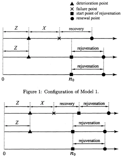
good as new, and the software ageis initiated at the beginning of the next highly robust state. Wecall theabovemodel Model1inthis paper. Figure 1illustrates the configuration

ofModel 1.

2.3 Model 2

Next, consider the other model. When the recovery operation is completed after the

system failure, it is assumedinModel 1thatthesystem is renewed and the stateismoved

to the highly robust state. However, since restarting the system after recovery operation

may require

some

cleanup and resuming the process execution at the checkpointed state,

asoftware rejuvenation after completing recovery operation will be needed to

renew

the system $[6, 7]$

.

Inthis case, the correpondingstochastic modelshould bedistinguished from

Model 1. We call this model in which the software rejuvenation is performed just after

the completion of recovery operation as well as at the prespecified time after the robust

state is entered, Model 2. Figure 2depicts the configurationof Model 2.

3. COST

EFFECTIVENESS ANALYSIS

Define the time lengthfrom the beginning of the system operation to the completion

of the preventiveor corrective maintenance as onecycle, and suppose thatthe same cycl

A deteriorationpoint

$\cross \mathrm{f}\mathrm{a}\mathrm{i}\mathrm{l}\mathrm{u}\mathrm{r}\mathrm{e}$point

$\blacksquare$ startpoint ofrejuvenation

\bullet renewalpoint

Figure 1: Configuration ofModel 1.

Figure 2: Configurationof Model 2.

is repeated again and againover an infinite time horizon. Then, themean operative time

during

one

cycle inModel 1is given by

$S_{1}(n_{0})$ $=$ $\sum_{n=0}^{n0-1}\overline{F_{f}*F_{0}}(n)$

.

(2)

The total expected cost for

one

cycle is obtained

as

Vi(no) $=c_{s}\mu_{a}F_{f}*F_{0}(n_{0})+c_{p}\mu_{cf}\overline{F}*F_{0}$(no). (3)

Then the cost effectiveness for Model 1is defined as the mean operative time per unit expected cost [13] as

$E_{1}(n_{0})=S_{1}(n_{0})/V_{1}(n_{0})$ (4)

and the problem is to seek the optimal software rejuvenation schedule $n_{0}^{*}$ maximizing it.

Takingthe difference of$E_{1}(n_{0})$ withrespect tonO, define thefollowingfunction $[13, 15]$:

$V_{1}(n_{0})V_{1}(n_{0}+1)$[$E_{1}(n0+1)-E_{1}$ n0-1

$q_{1}(n_{0})$ $=$

$\overline{F_{0}*F_{f}}(n_{0})$

$=$ $V_{1}(n_{0})-(c_{s}\mu_{a}-c_{p}\mu_{c})S_{1}(n_{0})r_{0f}(n_{0}+1)$, (5)

where $ff*f\mathrm{o}(n)$ is the pmf of the probability distribution$Ff*F_{0}(n)$

.

The following result gives the optimal software rejuvenation schedule for Model 1.

Theorem 1: For Model 1, (1) suppose that the probability distribution $F_{0}*F_{f}(n)$ is

strictly FR (increasingfailure rate) under the assumption $c_{s}\mu_{a}>c_{p}\mu_{c}$

.

(i) If$q_{1}(\infty)<0$, thenthereexist(at leastone, at mosttwo) optimal softwarerejuvenation

schedules $n_{0}^{*}(0<n_{0}^{*}<\infty)$ satisfying $q_{1}(n_{0}^{*}-1)>0$ and $q_{1}(n_{0}^{*})\leq 0$

.

Then, the

maximum cost effectiveness is given by

$\underline{E}_{1}(n_{0}^{*})\leq E_{1}(n_{0}^{*})<\overline{E}_{1}(n_{0}^{*})$, (6) where

$\underline{E}_{1}(n_{0}^{*})$ $=$ $\frac{1}{(c_{s}\mu_{a}-c_{p}\mu_{c})r(n_{0}^{*}+1)}$, (7)

$\overline{E}_{1}(n_{0}^{*})$ $=$ $\frac{1}{(c_{s}\mu_{a}-c_{p}\mu_{c})r(n_{0}^{*})}$

.

(8) (ii) If$q(\infty)\geq 0$, then the optimalsoftware rejuvenation schedule becomes $n_{0}^{*}arrow\infty$, $i.e$

.

it is optimal not to carry out the software rejuvenation. Then, the maximum cost

effectiveness is given by

$E_{1}( \infty)=\frac{\mu_{f}+\mu_{0}}{c_{s}\mu_{a}}$

.

(9)

(2) Suppose that the probability distribution $F0*Ff(n)$ is DFR (decreasing failurerate)

underthe assumption

_csfia

$>c_{p}\mu_{c}$

.

Then,thecosteffectiveness$E_{1}$(no) is

aconvex

function ofno, and the optimal software rejuvenation schedule is$n_{0}^{*}=0$

or

$n_{0}^{*}arrow\infty$

.

Next, consider Model 2. The

mean

length of operative time for

one

cycle and the total

expected cost during

one

cycle

are

given by

$S_{2}(n_{0})$ $=$ $\sum_{n=0}^{n_{0}-1}\overline{Ff*F_{0}}(n)$ (10) and

$V_{2}$(10) $=$ $c_{S}\mu aFf*F\mathrm{o}$(no)+CpMc, (11)

respectively. Then, the cost effectiveness for Model 2is formulated as

E2

$(n\mathrm{o})=S_{2}(n\mathrm{o})/V_{2}$(10) (12)

In afashion similar to Model 1, define the following function:

$q_{2}(n_{0})=V_{2}(n_{0})-c_{s}\mu_{a}r_{0f}(n0+1)S_{2}$(10) (13)

Theorem 2: For Model 2, (1) suppose that the probability distribution $F_{0}*Ff(n)$ is

strictly IFR.

(i) If$q_{2}(\infty)<0$, then there exist (at least one, at mosttwo) optimalsoftware rejuvenation

schedules $n_{0}^{*}(0<n_{0}^{*}<\infty)$ satisfying $q_{2}(n_{0}^{*}-1)>0$ and $q_{2}(n_{0}^{*})\leq 0$. Then, the

maximum cost effetiveness is given by

$\underline{E}_{2}(n_{0}^{*})\leq E_{2}(n_{0}^{*})<\overline{E}_{2}(n_{0}^{*})$, (11) where $\underline{E}_{2}(n_{0}^{*})$ $=$ $\frac{1}{c_{s}\mu_{a}r(n_{0}^{*}+1)}$, (15) 1 $\overline{E}_{2}(n_{0}^{*})$ $=$ (16) $c_{s}\mu_{a}r(n_{0}^{*})$

.

156

157

(ii) If$q_{2}(\infty)\geq 0$, thenthe optimal software rejuvenation schedule becomes$n_{0}^{*}arrow\infty$, and the maximum cost effectiveness is given by

$E_{2}( \infty)=\frac{\mu_{f}+\mu_{0}}{c_{p}\mu_{c}+c_{s}\mu_{a}}$

.

(17)

(2) Suppose that the probability distribution$F_{0^{*F}f(n)}$ isDFR. Then,thecost effectiveness

$E_{2}(n_{0})$ is aconvexfunction ofno,and theoptimalsoftwarerejuvenation schedule is$n_{0}^{*}=0$

or $n_{0}^{*}arrow\infty$.

4.

ESTIMATION ALGORITHMS

4.1 Graphical Method

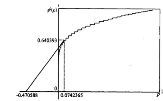
Forthe discrete $\mathrm{c}\mathrm{d}\mathrm{f}Ff*F_{0}(n)$, define thescaled DTTT transform $[6, 7]$:

$\phi(p)=\sum_{n=0}^{(F_{f}*F_{0})^{-1}(p)}\frac{\overline{F_{f}*F_{0}}(n)}{\mu_{f}+\mu 0}$, (18)

where

$(F_{f}*F_{0})^{-1}(p)= \min\{n : F_{f}*F_{0}(n)>p\}-1$, (19)

if the inverse function exists. Then it is evident that

$\mu_{f}+\mu 0=\sum_{n=0}^{\infty}\overline{F_{f}*F_{0}}(n)$

.

(20)

After afew algebraic manipulations,

we can

obtain the following result:

Theorem 3: For Model $i(i=1,2)$, obtaining the optimal software rejevenation schedule

$n_{0^{*}}$ maximizing the cost effectiveness $E_{i}(n\mathrm{o})$ is equivalent to obtaining $p^{*}(0\leq p^{*}\leq 1)$ such

as

$\max\underline{\phi(p)}$ ₍₂₁₎ $0\leq p\leq 1p+\beta_{i}$’

where $\beta_{1}=c_{p}\mu_{c}/(c_{s}\mu_{a}-c_{p}\mu_{c})$ and $\mathcal{B}_{2}=c_{p}\mu_{c}/c_{s}\mu_{a}$

.

Theorem 3is the dual ofTheorem 1and Theorem 2. From this result, it is

seen

that the

optimalsoftware rejuvenation schedule$n0^{*}=(Ff*F_{0})^{-1}(p^{*})$ isdetermined by calculating

the optimal point $p^{*}(0\leq p^{*}\leq 1)$ maximizing the tangent slope from the point $(-\beta_{i}, 0)$

$(i=1,2)$ to the curve $(p, \phi(p))\in[0,1]\cross[0,1]$ in the twodimensional plane.

4.2 Statistical Non-parametric Method

Next, suppose that the optimal software rejuvenation schedule has to be estimated

from $k$ ordered complete observations: $0=x_{0}\leq x_{1}\leq x_{2}\leq\cdots\leq xk$ of the times from

adiscrete $\mathrm{c}\mathrm{d}\mathrm{f}F_{0}*F_{f}(n)$, which is unknown. Then, the empirical distribution for this

sample, is given by

$F_{fk}(n)=\{$$i/k$ for

$x_{i}\leq n<x_{i+1}$, ₍₂₂₎

1for $x_{k}\leq n$

.

Then the numerical counterpart of the scaled DTTT transform, called the scaled DTTT

statistics, based on this sample, is defined by

$\phi_{ik}$ $=$ $\psi_{i}/\psi_{k}$, $i=0,1,2$ ,$\cdots$,$k$, (23)

Figure 3: Determination ofthe optimal software rejuvenation schedule for Model 1.

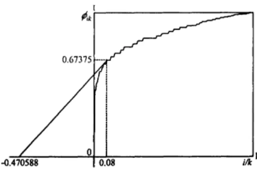
Figure 4: Determination of the optimalsoftware rejuvenation schedule for Model 2. where

$\psi_{i}$ $=$ $\sum_{j=1}^{i}(k-j+1)(x_{jj-1}-x)$, $i=1,2$,$\cdots$,$k;\psi_{0}=0$. (24)

The resulting stepfunction by plotting thepoints $(i/k, \phi_{ik})(i=0,1,2, \cdots, k)$ is called the scaled DTTT plot

The following theorem gives statistically non-parametric estimation algorithms for the

optimal software rejuvenation schedules.

Theorem4: Supposethat the optimalsoftwarerejuvenationschedulehasto beestimated from $k$orderedcomplete sample _{$0=x0\leq x_{1}\leq x_{2}\leq\cdots\leq xk$}ofthetimes from adiscrete

$\mathrm{c}\mathrm{d}\mathrm{f}Ff*F_{0}(n)$, whichisunknown. Then, anon-parametric estimatoroftheoptimalsoftware

rejuvenation schedule $\hat{n}_{0}^{*}$ which maximizes $E_{i}$(no) $(i=1,2)$ is given by

$x_{j}*$, where

$j^{*}= \{j|0\leq j\leq n\mathrm{m}\mathrm{a}\mathrm{x}\frac{\phi_{jk}}{j/k+\beta_{i}}\}$, $i=1,2$

.

(25)

5. NUMERICAL

EXAMPLES

5.1 Illustrative Examples

We present

some

examples to determine the optimal software rejuvenation schedule

which maximizes the cost effectiveness. Suppose that the time $X$ obeys the negative

binomial distribution with $\mathrm{p}\mathrm{m}\mathrm{f}$:

$ff(n)=(\begin{array}{ll}n -1r -1\end{array})$ $q^{r}(1-q)^{n-r}$, $n=1,2,3$,$\cdots$ , (24)

Figure 5: Estimation of the optimal software rejuvenation schedule for Model 1.

Figure 6: Estimation of the optimalsoftware rejuvenation schedule for Model 2. where $q\in(0,1)$ and $r=1,2$,$\cdots$ is the natural number. Also, it is assumed that $Z$ is

a

geometrically distributed random variable having $\mathrm{p}\mathrm{m}\mathrm{f}$:

$f_{0}(n)=p(1-p)^{n}$, $n=0,1,2$,$\cdots$

.

(27)

In the rest part of this section, we

assume

that $(r, q)=(10,0.3)$, $p=0.3$, $c_{s}=5.0\cross 10$

[$/day], $c_{p}=4.0\cross 10$ [$/day], $\mu_{a}=5.0$ [day] and $\mu_{c}=2.0$ [day].

Figures 3and 4illustrate the determination of the optimal software rejuvenation sched-ule on the two dimensional graph for Model 1and Model 2, respectively. Since $p^{*}=$

0.0742365 has the maximum slope from $(-\beta_{1},0)=$ (-0.470588, 0) in Fig. 3, the optimal

software rejuvenation schedule for Model 1is given by $n_{0}^{*}=(Ff*F\circ)^{-1}(0.0742365)$$=24$

.

On the otherhand, weobtain$n_{0}^{*}=(Ff*F_{0})^{-1}(0.0546002)$ $=23$inModel 2. In both cases,

the maximum cost effectiveness are given by $E_{1}(24)=0.246606$ and E2(23) $=0.233799$,

respectively.

Figures 5and6showtheestimation results oftheoptimalsoftware rejuvenation sched-ule for Model 1and Model 2, respectively, where the time data

are

generated from the negative binomial distribution. For 200 simulation data (negative binomial distributed random number), the estimates ofthe optimal rejuvenation schedule and its associated cost effectiveness are $\hat{n}_{0}^{*}=x_{17}=25$ and $E_{1}(\hat{n}_{0}^{*})=0.264209$ in Model 1. On the other

hand, one estimates $\hat{n}_{0}^{*}=x_{14}=24$ and $E_{2}(\hat{n}_{0}^{*})=0.246961$ in Model 2.

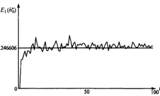
5.2 Asymptotic Behavior

Of our next interest is the investigation of the asymptotic behavior of the estimates

for the optimal software rejuvenation schedule. In Figs. 7 and 8, the estimates of the

maximum cost effectiveness are plotted where the horizontal line denotes the real

maxi-mum calculatedbased onthe negative binomial distributionwithsame parameters. Rom these figures, it is observed that the estimate of the cost effectiveness fluctuates around

thereal maximum and that the non-parametricmethod proposedhere

can

provideagood

Figure 7: Asymptotic behavior of the estimatesforthemaximumcosteffectiveness(Model 1).

Figure 8: Asymptotic behavior of the estimates for themaximumcost effectiveness (Model 2).

Acknowledgments: This research was partially supported by the Ministry of

Ed-ucation, Science, Sports and Culture, Grant-in-Aid for Scientific Research (B), Grant

No. 13480109 (2001), and the Research Program 2002 under the Institute for Advanced

Studiesofthe Hiroshima Shudo University, Hiroshima, Japan.

REFERENCES

[1] Adams, E. (1984), Optimizing preventive service of the software products, IBM

Journal

_of

Research aDevelopment, 28, 2-14.

[2] Avritzer, A. and Weyuker, E. J. (1997), Monitoringsmoothly degrading systems for

increased dependability, Empirical

_Software

Engineering, 2, 59-77.

[3] Bobbio, A., Sereno, M. and Anglano, C. (2001), Fine grained software degradation

models foroptimal rejuvenation policies,

_Perfor

mance

Evaluation, 46, 45-62.

[4] Castelli, V., Harper, R. E., Heidelberger, P., Hunter, S. W., Trivedi, K. S.,

Vaidyanathan, K. V. and Zeggert, W. P. (2001), Proactive management ofsoftware

aging, IBM Journal

_of

Research &Development, 45, 311-332.

[5] Dohi, T., $\mathrm{G}\mathrm{o}\check{\mathrm{s}}\mathrm{e}\mathrm{v}\mathrm{a}$-Popstojanova, K. and Trivedi, K. S. (2001), Estimating software

rejuvenation schedule in high

assurance

systems, The Computer Journal, 44 (6),

473-485.

[6] Dohi, T., Iwamoto, K., Okamura, H. andKaio, N. (2002), Discrete-time cost analysis

for atelecommunication billing application with rejuvenation, Proc. Second

EurO-Japanese Workshop onStochastic RiskModelling

_for

Fianance, Insurance, Production

and Reliability, 181-190

161

[7] Dohi, T., Iwamoto, K., Okamura, H. and Kaio, N. (2002), Discrete availability

models to rejuvenate atelecommunication billing application, Proc. lth IEEE Int’l

Symposium on High Assurance Systems Engineering, 159-166.

[8] Dohi, T., $\mathrm{G}\mathrm{o}\check{\mathrm{s}}\mathrm{e}\mathrm{v}\mathrm{a}$-Popstojanova, K., Vaidyanathan, K., Trivedi, K. S. and Osaki,

S. (2003), Software rejuvenation –modeling and applications, $Sp_{7}\dot{\mathrm{u}}nger$ Reliability

Engineering Handbook (H. Pham, ed.), Springer-Verlag, in press.

[9] Garg, S., Telek, M., Puliafito, A. and Trivedi, K. S. (1995), Analysisof software reju-venation using Markov regenerative stochastic Petri net, Proc. 6th Int’l Symposium

on

_Software

Reliability Engineering, 24-27.

[10] Garg, S., Pfening, S., Puliafito, A., Telek, M. and Trivedi, K. S. (1998), Analysis of

preventive maintenance in transactions based software systems, IEEE Transactions

on Computers, 47, 96-107.

[11] Gray, J. (1986), Whydo computers stop and what

can

bedone about it?, Proc. 5th

Int’l Symposium on Reliability in Distributed

_Software

and Database Systems, 3-12.

[12] Huang, Y., Kintala, C,Kolettin, N.and Funton,N. D. (1995), Softwarerejuvenation:

analysis, module and applications, Proc. 25th Int’l Symposium

on

Fault Tolerant

Computing,

381-390.

[13] Iwamoto, K.,Dohi, T., Okamura, H. and Kaio, N. (2003), Estimation ofdiscrete-time

software rejuvenation schedule based

on

thecost effectiveness,

Transactions

_of

IEICE

(A), in press.

[14] Liu, Y., Ma, Y., Han, J. J., Levendel, H. and Trivedi, K. S. (2002), Modeling and

analysisof software rejuvenation in cable modem termination syste

m,

Proc. 13thInt’l

Symp. on

_Software

Reliability Engineering, 159-170.

[15] Nakagawa, T. (1984), Asummaryof discrete replacement policies, European Journal

of

Operational Research, 17 (3), 382-392.

[16] Parnas, D. L. (1994), Softwareaging, Proc. 16thInt’l

_Conf.

on

Sof

tware Engineering,

279-287.

[17] Park,K. andKim, S. (2002), Availabilityanalysisandimprovementof$\mathrm{a}\mathrm{c}\mathrm{t}\mathrm{i}\mathrm{v}\mathrm{e}/\mathrm{s}\mathrm{t}\mathrm{a}\mathrm{n}\mathrm{d}\mathrm{b}\mathrm{y}$

cluster systems using software rejuvenation, Journal

of

Systems and Software, 61,

121-128.

[18] Pfening, S., Garg, S., Puliafito, A., Telek, M. and Trivedi, K. S. (1996), Optimal rejuvenation fortoleranting soft failure,

_Performance

Evaluation, 27/28, 491-506