Confidence Region Method for a Stochastic Programming Problem

Journal of the Operations Research Society of Japan

Vol. 30. No. 2. June 1987

CONFIDENCE REGION METHOD FOR A STOCHASTIC

PROGRAMMING PROBLEM

Hiroshi Morita, Hiroaki Ishii and Toshio Nishida

Osaka University

(Received June 12, 1986; Revised November 21, 1986)

Abstract We propose a minirnax model with a "quadratic" recourse. In stochastic linear programming models, a decision maker has been assumed to know the probability distribution of random variables. Here we consider the case that the parameters of distribution are unknown. We impose the restrictions on the unknown parameters from the view point of a confidence region, and then seek a minimax solution that minimizes the worst case of the parameters. This model reflects the situation minimizing the maximal possible damage. Especially, the independent normal distribution model is discussed in detail. The analysis for a sufficiently large sample size and a numerical result are given.

1. Introduction

The elements of coefficient matrices of linear programming problems have been assumed to be exactly known. However, in a real life, we never know these values with the full conviction, so we have to include the uncertainty in the formulation of the practical problems. In a usual stochastic pro-gramming problem, this uncertainty is viewed as a random model characterized by a probability distribution, and in order to solve the problems under un-certainty, several approaches have been proposed, e.g., two-stage stochastic programs with recourse [6J, chance-constrained stochastic programs Ll) and so on. In most of these approaches it is assumed that the probability dis-tributions of the random variables are perfectly known. But when the param-eters of distributions are unknown, we can not apply these approaches as they are. In this situation we need to obtain some knowledge about the para.meters of distributions in statistical ways. Jagannathan [3j proposed an approach

218

Stochastic Program by Confidence Region 219

with sample informations for a given prior distribution of unknown parameters using a Bayesian approach.

Here we propose a so-called game theoretic minimax approach in section 2. First we impose the restrictions on the unknown parameters which are estimated by a confidence region of the,m based on random samples drawn from a parent population, and then we seek a minimax solution that minimizes the worst case of the parameters among those restrictions, that is, we minimize the maximal possible damage for a given significance level. In section 3, we investigate the independent normal distribution model in detail. The minimax model is solved numerically using some properties, and the discussion of limiting property is added. Finally we show a numerical example in sec-tion 4.

2.

Formulation of a Minimax Model

A linear stochastic programming problem is given as follows:

(2.1) LP: Minimize _x c t x

subject to Ax = b,

where c and ;r; are n real vectors, b is an m real vector and A is an m by n real matrix with a full rank. Here we assume that A and c are exactly known and b is a random vector having a distribution function F(·;8) where 8 is an unknown parameter vector. We consider the following two-stage stochastic programming problem

Po

with a "quadratic" recourse:

(2.2) c t x

+

E(

m

I

d.y.) 2

i=1

1-

1-subject to Ax

+

Y = b, where d=(d

1,d2, ••• ,dm), weight of each constraint infeasibility, is an m-vector with positive elements, and Ai is an i-th row of matrix A. The quad-ratic recourse is more tractable than a simple recourse in this model and reflects the situation that the infeasibility of constraint has a critical meaning.

(2.3) P ' •

_o·

is rewritten to the following problem

m 2 Min1mize ctx

+

Er

I

d.(A.x-·b.) ]

i=1

1- 1- 1-P ' •

_o·

ctx

+

f···f

I

_{d.(A.X-t.)2 dF (t 1,t2,···,t ;8)}

i=1

1- 1- 1- m

The unknown parameter 8 is imposed the restrictions estimated by the con-fidence region S witn a certain significance level. We consider the worst case of the parameter 8 among S, and then minimize the objective function of

220 H. Morita & H. Ishii & T. Nishida

That is, we propose a following minimax model P:

(2.4) P: Min~mize L

=

ctx

+

max

f···f

I

d.(A.x-t.)2x

6£S

i=1

~ ~ ~

This model reflects on the situation that we should make a decision mlnimiz-ing the maximal possible damage if the correct value of the parameter 6 is not known perfectly.

3. Normal Distribution Model

Let

b

i

, i=I, ...

,m, be an independently, normally distributed random

var-iable, respectively. First we construct the confidence region S of parame-ters (i.e., mean and variance). For this purpose, we define the following notations. ~i mean of b

i

, i=I, ...

,m 2 cri variance of b

i

, i=I, ...

,m ~i sample mean of b

i

, i=I, ...

,m 2

si

sample variance of b

i

, i=I, ...

,m N sample size a significance level (%)

~(.): probability density function of independent multivariate stan-dard normal distribution

3.1. ,Confi dence regi on of parameters

(i) Confidence region of mean ~.,

i=I, ...

,m ~

Note that the distribution of Hotelling statistics, F,

- 2 N(N-m) m (~.-~.) \' '~ ~ (3.1) F L m(N-l)

i=1

s~

~

is the F-distribution with (m,N-m) degrees of freedom. Using this statistics F, the

(3.2)

confidence region of ~.,

i=I, ...

,m, is

- 2 ~ m (~.-~.) m(N-l)

I

~ ~

:;:

i=1

s~

~ N(N-m) F (m,N-m), a given by where F a("') is an a percintile of F-distribution. (ii) Confidence region of variance

cr~, i=I, ... ,m

~

Stochastic Program by Confidence Region 221

variance-covariance matrix. we find it approximately by that of each variance for an independent case. The distribution of

(N-I)s~/cr~

is the chi-square

1- 1- .

distribution with (N-I) degrees of freedom. Therefore the confidence region

2 of 0i' i=I •••. • m. is 2 (N-I)si =< 0_2. (3.3) - 2 - - - 1-given by 2 (N-I)si

Xs

(N-I) ::;; 2 X_I -S (N-I) i=I •... • m.

where S =

i

aI/m and

Xs (.)

2 is a S percentile of chi-square distribution. Then this region is a rectangular region.

From (i) and (H). the confidence region S is

(3.4)

{

I

m (jJ

.'-~.)

2 m(N-I) S

=

(jJ .•

o~).

i=I ••..• m

I

~---21-

::;; - - - F (m.N-m). 1- 1-

i=1

s. N(N-m) a

1-(N-I)s~

(N-I)s~

} ~ ____ ~1- ::;; 02 ::;; 1- i=I •••.• m. 2 i 2 XS(N-I) X I_8(N-I)

3.2.

Minimax model

We consider the maximizing part of minimax model P under the above set-ting. Le .• (3.5) P' : Maximize (jJ.,o~)e:S 1- 1-m 2 2

I

{d.(A.x-jJ.)

+

d.o.}. i=1 1- 1- 1-

1-Moreover this problem pr is divided into the following two problems:

(3.6) (3.7) Maximize o. 1-subject to Maximize jJ. 1-subject to m

I

i=1

2 (N-I)s. 1-m 2

Id.

(A .X-jJ .)

i=1

1- 1- 1-i=I, ••• ,m. - 2 (jJ.-jJ.) 1- 1---=-2-'-- ::;; s. 1-m(N-I) F (m,N-m)

~

K N(N-m) a

Then PI corresponds to the variances and P

2 corresponds to the means. Since maximum of P

l is independent of x, we Dlay regard it as a constant in a

mini-mizing of P with respect to

x.

Hence we consider only P 2. In order to solve p. we show the several properties.

222 H. Morita & H. Ishii & T. Nishida

Property 1.

L2 is maximized on the boundary of the feasible region, and further the sign of (~~-~.) is opposite to that of (A.x-~.), where ~~ is

1.- 1.- 1.- 1.-

1.-an optimum of ~i'

i=l, ...

,m.

Proof:

It is easily shown that L2 is a convex function in every ~i'

i=

1, ..• ,m, and so the first part of property 1 is proved directly by the theory of convexity. Actually, L2 is maximized when

* -

2 (~.-~.) 2 (3.8) 1.- 2 1.- K • 1

i

,

1.-= , ••• ,m, s. 1.-that is, (3.9) m where K.

~

°

and

L

K~

=

K. 1.-

i=l

1.-imizes L2 is given as follows:

*

~

.

-

s .K. i f A.x-~ . ~ 0, ~

.

(3.10) 1.- 1.- 1.- 1.- 1.-

1.-*

+

s.K. i f A.x-~ . < 0. ~

.

~. 1.- 1.- 1.- 1.- 1.- 1.-

0

Property 2.

P

2 is transformed into a concave programming problem

Pi

by making (3.11) a variable transformation: - 2 (~.-~.) z. = 1.-1.- 1.- • 2 ' 1.-=l, ••• ,m. s.

1.-Proof:

From (3.13) d .s

.1

A .x-~

.1

1.- 1.- 1.- 1.-2 z~/2 < 0,

1.-Li is a concave function. Therefore property 2 follows from property 1.

Solving

(3.14)

Pi,

the optimand

2 2 - 2

disi(Aix-~i)

2 2 (A-d.s.)

1.-i=l, ...

,m, is expressed as follows:

where A is the Lagrange multiplier of Li.

Property 3.

A is the largest solution of the equation

m (3.15)

L

i=l

2 2 - 2 disi(Aix-~i) 2 2 (A-d.s.) 1.-K.

Proof:

Denoting the maximum value of Li with L;(A),

Stochilstic Program by Confidence Region

(3.16) L~(A) m

I

d . (A.X-]J .) _

2[ A )2

- - 2 .

i=l ~ ~ ~ A-d.s:

~ ~

Let AI' A2 (AI < A₂) be solutions of eq.(3.15), then

(3.17)

d.s~

~ - 2 ~ ~ L d. (A .x-]J .) ---;2:---;:"2 "'=1 _" ~ ~ ~ (' _1\2-d _.s. ) ~ ~ Therefore, from eq.(3.17),

(3.18) 2 2 - 2 m disi(AiX-]Ji) (A₁+A_{2) )} 22 2;':= ~=1 (A1-dis i ) (A2-disi ) m 2

I

i=1 3 4 - 2 d.s. (A .x-]J.) ~ ~ ~ ~ 2 2 2 2 (A 1-d.s.) ~ ~ (A2-d.s.) ~ ~ > 0 . 2 2 2 2 (A 1-d.s.) ~ ~ (A2-d.s.) ~ ~ Hence A is a largest solution of eq.(3.15).

223

o

Property

4.

A > AO

~

max

dis~,

where I is the set of indices such that iEl

A.x-~. '" _{~ ~} O.

Proof:

From eq.(3.15), we define

(3.20) Since (3.21) (3.22) and (3.23) G(A) ~ m

I

i=l lim G(A) A-+~+O lim G(A) A-++')O 2 2 - 2 d.s.(A.x-]J.) ~ ~ ~ ~ 2 2 (A-d.s.) ~ ~ +00 >0, - K < 0, G'(A) = -2

I

iEl - K. > 0,

the unique solution exists in (AO'oo).

Consequently, the problem P is expressed as follows:

(3.24) p' : Minimize

x,A

subject to

224 _{H. Morita & H. Ishii & T. Nishida}

where we neglect the constant associated with Pl.t In order to solve this problem pI, we utilize the following property.

Property 5.

For A

~ ~

Aa' pI is a convex programming problem.

Proof:

It is sufficient to show that the Hessian matrix of the objective function is positive semi-definite for A

~ ~

Aa' The elements of the Hessian matrix, H=(h .. ), i,j=l, ..• ,n+l, are given as follows:

1-J (3.25) h .. 1-J h . n+l,1- h. 1-,n+l 2 , k=l, •..• ,n,

where a .. denotes the (i"j)-th element of matrix A. Note that H is divided 1-J

into two matrices, that is,

where ~i' i=l, •.. ,n, and ~ are m-vectors with

~ - 2 2v2d .(A.x-Il.)d.s.

I2d':"

A _ J _

A-d.s~

J J a .. , and J1-J J J J J 2 2 (A-d .s .) J J

as j-th element, j=l, ••. ,m, respectively, and

(3.27) w =

m

2

I

k=l

Since for A

~ ~

Aa' w is non-negative, H is expressed as the sum of two posi-tive semi-definite matrices. Therefore H is positive semi-definite.

0

In order to solve this problem pI, we should consider several cases according to the value of A because of the dependency on x. Define

(3.28) A max max l:£i:£n Case 1. A

~

1.

A 2 max

d.s~

1-Since it is clear that Aa :£ Amax' from property 5, the problem pI is a convex program. Then we use some approaches for a constrained non-linear programming problem, e.g., the steepest descent method with a penalty

func-t It is pointed out by the referee that the problem (3.24) which is equiva-lent to the problem (3.7) is also found by a duslity theorem

L2,

Theorem 2.l.j. We summarize it in appendix.

Stochastic Program by Confidence Region

tion.

Case 2. Aa < A <

1

Amax

For fixed A, L is convex with respect to x. Then, for several fixed A between Aa and -23 A , we seek optimal solutions and choose the best ones

max

among them. But we must divide A into the following some intervals because 225

the constraints differ on each interval. For a sake of convenience, we

rear-2

range dis_i, i=1, •.• ,m, in an increasing order with its constraint. By the definition of Aa'

(3.29) Aa d s2 mm means

0.3a) A.x of _{lli' i=1, ...} ,m,

<-and

0.31) _Aa d _pSp' 2 for 1~p<m,

means

A.x of _{lli' i=1, ... ,p,} (3.32)

<-Aix lli' i=p+l; ... ,m.

2

Thus p denotes the largest index such that Aix of lli' For Aa

=

dps

p' l~p<m, the first constraint of pI is relaxed as follows by a way of compensation that the equality constraints A.x = ~., i=p+1, ... ,m, are imposed. Moreover,

<-

<-since rank A

=

n, the constraints eq.(3.32) should be infeasible for p<m-n. That is, the constraints of problem pI are partitioned into n cases as fol-lows. (3.33) and (3.34)

I

i=1 2 2 - 2 d.s. (A.X-ll.) 1, <- <- <-2 <-2 (A-d.s.)

<-=

K, A.x <- ~i' i=p+1, ... ,m, d s2

P

p m

L

i=1 2 2 - 2 d.s. (A.X-ll.) 1.<- <- <-2 <-2 (A-d.s.) <-d s2 < A <

1

A m m 2 max' K, for p

=

m.

Hence we need to obtain an optimal solution for every p.

Choosing the best optimal solution among optimal ones of above two cases, we obtain the global optimal solutions. Next we show the existance of this best optimal solution.

226 H. Morita & H. Ishii & T. Nishida

Lemma 1.

The objective function L is bounded subject to eq.(3.33) or eq. (3.34).

Proof:

Assum that the optimal solution is unbounded, then since the denominator of the first constraint is bounded, the left hand side of it must

be unbounded. This contradicts boundness of K.

_o

Lemma 2.

The solution od p' is continuous with respect to A.

Proof:

Let xl and x₂ be optimal solutions when

A

=

Al

and

A A

_Z

'

re-spectively. It is easily shown that L(X

l) ~ L(X

2

)

as

A2

~

Al

and the solution is unique because this problem has a strictly convex objective function and a convex feasible region for fixed A. From this convexity the continuity of

the solution is shown.

0

We can find the solution of this problem approximately with discretizing value of A.

Theorem.

We can obtain the approximately global optimal solution by means of choosing the best optimal solution among optimal ones for each discretized

A.

3.3. Limiting property

We discuss the problem with sufficiently large sample size. We see, from a consistency of sample mean and variance, that the correct value of parame-ters can be known as N~oo. With these parameters, Po is rewritten to a problem PL with perfect information as follows:

(3.35) PL: Minimize

x

Ct _ ~,

+

m

I

{d.(A.x-~.) 2 + d.a.}. 2 i=1 ~ ~ ~ ~ ~

Here we show that our proposed model with finite sampling with size N, say P, tends to PL as N~oo.

Lemma 3.

Let M and N be positive integers, then

X~(N)

(3.36) lim - -

=

1 and (3.37) N~oo N Fex(M,N) lim -N~oo N where 0 < ex < 1. 0,

Proof:

As in

[4J,

with the Cornish-Fisher expansion,

(3.38)

=

U

et

+

0(_1_),

IN

where Uex is ex percentile of a standard normal distribution. Since lu

I

< 00,

Stochastic Program by Confidence Region 227

for 0 < ~ < 1, eq.(3.36) is proved.

Denoting the probability density function of F-distribution with (M,oo) degrees of freedom with fM oo(t),

, M

f (t) = _1_

(~

te- t

)2

M,oo r(~) 2

2

(3.39)

it is clear that an ~ percentile of this distribution, F~(M,oo), finitely

ex-ists. [J

Remark 1.

From lemma 3, the problem P with unknoWn parameters tends to the problem PL with known parameters as a sample size N tends to infinity.

Remark 2.

In the problem pI, A tends to infinity as N+oo.

Remark

3. Note that sample variances are not concerned with a decision making for a sufficiently large sample size. They are concerned with only the magnitude of the recourse.

Remark 4.

This proposed minimax model would be useful to the other sto-chastic programming problems which the parameters of their random variables are unknown.

4. Numerical Example

Consider a following problem:

(4.1) PE: Minimize 2x 1

+

x2 X₁'X₂ sUbject to _Xl

+

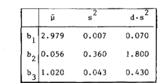
X 2 b1 2x 1 - X2 b2 X 2 b3 where b

1, b2 and b3 are independently, normally distributed random variables with unknown parameters, and let a weight vector d = (10,5,10). Using an artificial result of sampling of a computer simulation, we give the sample means and variances in Table 1.

Table 1. Sample means and variances (N=ll)

ii s 2 d·s 2 b l 2.979 0.007 0.070 b 2 0.056 0.360 1.800 b 1.020 0.043 0.430

228 H. Morita & H. Ishii & T. Nishida

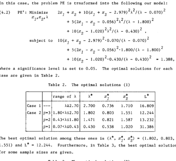
In this case, the problem PE is trnsformed into the following our model:

(4.2) PE': Minimize x₁₃x₂₃ A subject to 2 2 ') 2x₁

+

x₂

+

10(X₁

+

x₂ - 2.979) A /(A - 0.070)~ 2 2 2

+

5(2X₁ - x₂ - 0.056) A /(A - 1.800)

+

10(X 2 - 1.020)2 A2/(A - 0.430)2 , 2 2 10(X_l

+

x₂ - 2.979) ·0.070/(A - 0.070) 2 2

+

5(2x₁ - x₂ - 0.056) ·1.800/(A - 1.800)

+

10(X 2 - 1.020)2· 0 . 430 /(A - 0.430)2

=

1.388,

where a significance level is set to 0.05. The optimal solutions for each case are given in Table 2.

Table 2. The optimal solutions (1)

range of A A* x* 1 x* 2 L* Case 1 - - - A<:2.70 2.700 0.736 1. 710 16.809 Case 2 p=3 1.80<A~2. 70 1. 802 0.803 1. 551 12.244 p=2 0.43<A~1.80 1. 471 0.821 1. 587 13.232 p=l 0.07<A~0.43 0.430 0.538 1.020 31. 386

The best optimal solution among these ones is (A*, x~, x~)

=

(1.802, 0.803, 1.551) and L*

=

12.244. Fourthermore, in Table 3, the best optimal solutions for some sample sizes are given.

Table 3. The optimal solutions (2)

N A* _xl * x* 2 L* 11 1.802 0.803 1. 551 12.244 100 5.870 0.825 1. 710 11. 355 300 8.642 0.820 1.649 10.640 1000 16.270 0.840 1. 651 10.271 00

-

_{0.967 1.695 9.887}

5.

Conclusion

We have proposed a minimax model. When the distribution of parameters of random variables are assumed to be unknown, our approach is seemed to be not only reasonable but useful. It notes that the maximizing process with respect to variances does not affect upon an optimal decision of our model

Stochastic Program by Conruience Region 229

though they are unknown. Fourthermore we show that, for a sufficiently large sample size, our model tends to one with .a perfect information. Hereafter the better solving algorithm should be considered. But it is ascertained the non-convexity of the objective function by a simulation, so it is remained a difficulty on solving our model.

Appendix.

Derivation of Problem

pi

by a Duality Theorem

The problem (3.34) pI which is equivalent to the problem (2.4) p for a

normal model is also derived by a duality theorem

[2].

To solve the maximiz-ing process of minimax problem P, it is sufficient to consider only the prob-lem (3.7) P2' From L2, Theorem 2.lj, - 2 m

_I

2)

m (~.-~.)

K}

d .(A.x-~.)

I

_'1.-_ _ ~ - ~ i=1 '1.- '1.- '1.- i=1 s~ (A. I)

'1.-inf {sup

{L(~,A)

A ~i - 2 m 2 m (~.-~.)

I

=

I

d.(A.x-~.)

+

A(K -

I

'1.- 2'1.- )} i=1 '1.- ~ '1.- i=1 $. '1.-Then for A > Aa, L(~,A) is maximized at ~i ~i' i = I , ••• ,m, where

(A.2) and (A.3) - 2 A~.- d.s.A.x '1.- '1.- '1.- '1.-L(~, A) A -

d.s~

'1.- '1.-m AK

+

I

i=1 A -

d.s~

'1.- '1.-From dL(~,A)/dA

=

0, m (A.4) K

I

i=1 and (A.5) L(~,A) 2 2 - 2 d.s.(A.x-~.) '1.- '1.- '1.- 'Z-2 'Z-2 (A-d.s.) '1.- '1.-A ) 2 2 • d.s. 'Z-

'Z-Therefore the problem (3.24) pI is obtained, where the constraint A > Aa is found from property 4.

230 H Morita & H. Ishii & T. Nishida

Acknowledgements

The authors would like to thank the referees for their valuable c:omments made on this paper.

References

[lJ

Charnes, A. and Cooper, W. W.: Chance constrained programming. Manage-ment Science, Vol.6, No.1 (1960), 73-79.

[2] Isii, K.: Inequalities of the types of Chebyshev and Cramer-Rao and math-ematical programming, Annals of Institute Statistical Mathematics, Vol. 16 (1964), 277-293.

[3] Jagannathan, J.: Use of sample information in stochastic recourse and chance-constrained programming models, Management Science, Vol.31, No.1

(1985), 96-108.

[4J Takeuchi, K.: Approximation of probability distribution, Kyoiku-shuppan, 1973, (in Japanease).

[5J Vajda, S.: Probabilistic programming, Academic Press, 1972.

[6j Walkup, D. W. and Wets, R.: Stochastic programs with recourse, SIAM Jour-nal of Applied Mathematics, Vol.15 (1967), 1299-1314.

Hiroshi MORI TA: Department of Applied Physics, Faculty of Engineering, Osaka University, Yamada-Oka, Suita, Osaka, 565, Japan.