BOND PORTFOLIO OPTIMIZATION PROBLEMS AND THEIR APPLICATIONS TO INDEX TRACKING:A PARTIAL OPTIMIZATION APPROACH

(1)

Journal of the Operations Research Society of Japan

Vol. 39, No. 3, September 1996

BOND PORTFOLIO OPTIMIZATION PROBLEMS A N D THEIR APPLICATIONS TO INDEX TRACKING:

A PARTIAL OPTIMIZATION APPROACH

Hiroshi Konno Hidetoshi Watanabe Tokyo Institute of Technology

(Received March 1, 1994; Final October 25, 1995)

Abstract We will discuss exact and efficient parametric simplex algorithms for solving a class of nonconvex minimization problems associated with bond portfolio optimization models which one of authors proposed in the late 1980's. We will show that globally optimal solutions of both total and partial optimization problems can now be calculated on a real time basis. Also we will present some computational results of a partial optimization model applied to a tracking of an index portfolio.

1 Introduction

In the late 1980's. one of the autllois proposed a pair of bond portfolio optimization models taking into account a variety of objectives and constraints associated with the dealing activities of bond managers of institutional investors.[7].

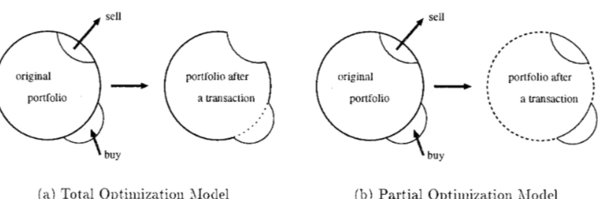
Of the two models, one is the "total" optimization moclel which intends to optimize (either maximize or minimize) a certain index associated with a total portfolio after a transaction (Fig l ( a ) ) . This model was formulated as a bilinear fractional programming problem, whose good locally optimal solution (which may or may not be a globally optimal solution) can be calculated reasonably fast by a heuristic algorithm based upon the simplex method for lineal programming problems. Hence. this model has been used in practice by several institutional investors both in Japan and in U.S..

The "partial" ~ptirnizat~ion model. on the other hand tries t o optimize the difference of a given index associated with the bundle of assets purchased from the market and sold to the market (Fig l @ ) ) . Though odd looking from a viewpoint of standard approach in portfolio optimization, partial optimization is often considered more attractive from the viewpoint of practitioners as evidenced by a series of interviews with a number of bond managers of institutional investors. The primary reason is that only a small fraction, typically less than 10% of the total assets on-ued by an investor is sold ancl/or purchased in a typical transaction.

Therefore the resulting improvement of the 013 ject ive function before and aft er a trans-

action in terms of tot,al optimization moclel is very small since at least 90% of the assets remains the same, while the improvement in terms of partial optimization model can be very significant. In fact. the competence of a bond manager is appreciated more in terms of partial optimization than tot a1 optimization.

Unfortunately. however this pal tial optimization moclel results in a difficult nonconvex minimization problem. for which the antlior could not devise an exact and efficient algorithm ill ['i] and thus this moclel was not used in practice until recently.

(2)

sell original

-

portfolio buy portfolio after a transaction portfolio after \ , a transaction '

-.

( a ) Total Optimization Model (11) Partial Optimization Model

Figure 1: Bond Port ofolio Optimization Models

The purpose of this paper is to demonstrate that this nonconvex minimization problem resulting from the partial optimization moclel can be solved to global opt imality very fast as a result of recent clevelopmeiits in global optimization methods [G]. In fact they can be solved in approximately the same amount of computation time as that needed for solving a linear programming problem of tlie same size. This means that we can solve both total and partial optimization models on a real time basis.

The readers will find that the model developed in this paper is different from tlie classical and st andarcl bond port folio optimization models in which the portfolio is constructed so as to meet the (fixed) future cash flows with minimal cost under the assumption that tlie investor holds the portfolio until maturity. (The readers are referred to the standard text such as Elton-Gruber [4] and Fong-Fabozzi 151. for conventional models.

To the contrary. the moclel developed in this paper is concerned with the dealing of bonds where the portfolio manager tries to hold a portfolio with maximal performance index in an effort to maximize his or her profit. We believe that this kind of model would play more and more important roles in bond dealing business and bond management associated with asset allocation.

In the next sect ion. we will explain several basic not ions associated wit 11 bond port folio management. In section 3. we will introduce tot a1 and partial optimization models. Sec- tion 4 will be devoted to exact and fast algorithms for solving these moclels which is based upon a variant of parametric simplex algorithm [g] for solving a class of global optimization problems. Finally in Section 5. we show some preliminary results of our numerical experiments using the historical clat a of government bonds available in the marliet . Here we will concentrate on the application of partial optimization moclel t o index tracking.

2 Bond Portfolio Optimization Models

Let us assume that an investor holds u, units of bonds

BA

j = 1. . . . . / I ) . Associated with B, are four basic at tributes[4.5.7].

5:

coupon to be paid at a fixed rate (yen/l~oiicl/year)

f"

: principal value to be refunded at maturity (yen/bond)

11,: unit transaction price in the marliet (yen/bond)

t,:

maturity (number of years until the principal value is refunded)

It is well lillown that if the interest rate i remains constant t,l~roughout the life of a bond, then the theoretical price 11, of

B,

is given by the following formula:

(3)

Bond Portfolio Optimization

l.,

l), = C l +

f.

( l

+

i ) t ( l

+

i ) ' ~

To emphasize the dependence of p, on the interest rate i. we employ an alteinative not at ion p, ( i ) i11 the sequel. The duration and conwxity of B, are then defined as follows:

c / , ( / ) = - p ' { i ) / p ( i ) ( 2

C,(i) = p"i))/p(i) ( 3 )

In reality however. the interest rate varies from period to period. Under such drcum- stances. the theoretical price of bond ( 1 ) has t o be replaced by taking its fluctuation into account. Let T = max

f,

and let

c,,

be the cash flow from

B,

during period

t .

Then tlie

l<,<"

theoretical bond price is give11 by

(17

where it is the interest rate to be applied during period f ( I = 1. . . . . T ) . Also the duration

d j and C, has to be replaced by

1 . rf,(ii. . . . . i r ) = - P , ( / ~ . . . . . i r ) / l ) , ( i i . . . . . i T ) where 1 . . y),(il

+

Ai. . . . . ir

+

A / ) - p j ( i l , . . . . i T ) p , ( i l . . . . . i r ) = 11111 AI-o Ai p ' ( i i

+

Al..

. . . IT

+

A i ) - p ' ( i l . . . . . i T ) . . . i T ) = lim A(-o Ai

Let us note that tlie term structure ( i i . . . l T ) can be calculated very fast by using several

efficient met hods iiiclucliilg[8] .

Bond managers of institutional investors. when evaluating a portfolio 11 = ( u l . . . . . u , ? )

take into account such performance indices as: ( a ) average unit price 7r( 1 1 )

(11) average direct yield (average coupon rate) c ( u )

77 n

( c ) average maturity

t (

U )

?? 77

(cl) average duration cl( 21) r1

( e ) average convexit'y

C{u}

(4)

Most fund managers prefer to liave a portfolio v-it11 larger average unit price and average direct yield. Also many. if not all managers. prefer to liave a shorter average maturity. because a larger risk is associated witli a portfolio with a longer maturity. Furtliei they prefer to have average duration and average convexity to remain within a certain interval to avoid risk associated witli the flnct uatioii of interest rates.

Ill addition to five indices listed above. most fund managers want to have larger average yield to maturity. to be defined below. The traditional definition of yield to maturity of a bond B, is the smallest iionnegat ive solution of the following nonlinear equation:

t~

A ( I + s ) ' - ' =

x c J ( l + ~ t

+ f J t=l

where pi is the price of B, in the "market. Instead. we will employ an alternative (and more meaningful) definition:

f l

14(1+v,)" = Z c , ( l + i l ) - - ( l + i t ) +

f,

t=l

( 9 ) The left hand side is tlie total amount of cash obtained by saving

p,

at the compound annual interest rate v, until maturity v\-liile the riglit hand side is tlie total amount of cash obt aiiiecl by saving all coupon payments under tlie interest rate structure

6

( t = 1. . . . . t, ) plus tlie principal value. The average effective yield v ( u ) of a portfolio 11 is defined as follows:

( f ) Average effective yielcl U ( 1 1 )

n n

v(u) =

EvJ1'J1'J/

E ~ J ~ L v ,

]=l ]=l

( 1 0 )

It is easy to see tliat the trader will get the effective yield U ( Ã ‡ per period by holding a

portfolio ( 11 1. . . ). Thus lie or she prefers t o have larger average effective yielcl.

3 Mathematical Description of Bond Portfolio Optimization Models.

Let us assume again that an ii~vest~or holds 11, units of By. ( j = 1 , . . . , U ) out of which 11 1 are

chosen as candidates for sale in tlie market. In a typical situation, n is a few hundred and nl is less than one hundred. Also let us assume tliat units of bond B g k = 1. . . . . U ? )

are available in the marliet . The bond trader sells

B]

( J = l , . . . . / x i ) to tlie market and

purchases B from the market to improve a portfolio. In a typical situation. he chooses a particular index out of (a)-(f) explained in Section 2 and tries to optimize (either maximize or minimize) it while putting others into const raint S by specifying the least desirable level

for each of them.

Let .Q = amount of B, to be sold. J = 1 , . . . , ~1 _{( 1 1 )}

AYk = amount of

B

'

to be purchased, k = 1.. . . , n ; ( 1 2 )

These variables liave t o satisfy the conclit ions:

O

5

.Q 5 (lJ. ,j = l . . . . . rll ₍₁₃₎

0

<Xk

5 k = l . . . ~ ? ( 1 4 )

In addition to these. several constraints are associated \vit 11 transact ions such as the restrictions on tlie total amount of bonds to be sold and/or purchased, total amount of profit and/or loss and the total amount of liquidation, all of which are represented as a linear function of

.q

'S and

Xi.

'S.

Let 11s note tliat all of indices (a)-(f) as well as the constraints above belong to a class of linear or bilinear fractional functions of u if the price pi "s are constants. Unfoi tnnately. however some of p, ' S are variables rather than constants in a typical transaction environ-

(5)

Bond Portfolio Optimization 299

entitled to choose the price of each bond within a certain interval provided the agent agrees to this transaction. The reason why a trader agrees to sell a bond B, for the price lower than the market price

p,

is that he wants to reduce the amount of profit (difference between selling price

p,

and the book price p,J out of this transact~ion. thereby reduce the amount of tax. The agent may instead agree t o sell another bond. B',. for the price lower than the market price Pk to compensate a loss of the trader. The transaction price is. however not permitted to deviate more than a few percent from the reference price due to a regulation imposed by the government.

Let 9, and

h

be the unit transaction price of B, and B',,. respectively. They have to satisfy

( 1 - A,)pj

<y,

5

( 1

+

A j ) p j , j = l . . . . , H I (15)

( 1 - \',.)Pk

<

f i

<

(1

+

A;,)Pk. k = 1 . . . . ,122 ₍₁₆₎

where p, and Pi, are the price of B, and B',, , respectively in the market and A, and AL are constants called "price adjustment coefficient S" . Thus a generic tot a1 opt imizat,ion model

71 can be formulated as follows:

This model would serve as a reference model when a, significant portion, say more t8han one third of the assets owned by an investor is subject t o sale.

Let us note that we can assume without loss of generality that the divisors of the frac- t,ional tjerms of the objective function and constraints are positive for all solutions satisfying other constraints. Therefore the problem (P) is equivalent t o the following bilinear fractional programming problem: j=l k= l maximize

_"

₁ _{" 2} T O -

^ p j

+

r',y,).t,

+

^( Ri.

+

R;.rt)-\-L i=l k= l

"

1 ni

subject t'o

3, <

+

y'jy^.rj

+

^(Gii-

+

G;;.yi.)-~k 5 d,, i = 1, . . .

,

(18)

,=l k=l

0

5

.r,

^

11,.

'$

5

u,

J = l . . . . - I l l

(6)

Let us now turn to the partial optimization model. the main topic of this paper in which the difference of a given objective. say O1 associated with the bundle of assets (A'l,. . . , ₎

purchased from the marliet and . . . . .I.,,, ) sold to the market subject to the same con-

straints as (18) (See Fig l(]))). This means that we evaluate the objective and constraints relative to the total portfolio owned by an investor after the transact ion except the objective

01 .

The problem can now be formulated as follows:

where k= l _-j=l maximize ,,? 71 1 ^ ( R ,

+

R m i , x ( r j

+

r;,yj).rj A-= l j=l 77 Â¥ " 1

subject t o

J,

5

^(G,(.

+

G>t.).\\.

+

g;,gJ.r,

5 a,.

i = 1. . . nil (19)

as before. we will assume that the divisors of the objective functions are positive for all feasible solutions. Also. we assume that the divisors in the objective funct,ion are of similar magnitude. so that it is meaningful to compare the difference. A typical example is the one explained is Section 5 in which the variables ( x i , . . . . ~ r I l 1 ) and (A'l, . . .

,

A'n, ) are constrained so that

This means that the total amount of cash spent for purchasing t,he portfolio (AF1. . . ,Yn2) is the total amount of cash from the sale of the portfolio ( ~ 1 , . . . , X , , , ) plus the income C from

the coupon payment during the given period. It then follows that divisors of performance index (a)-(f) associated with portfolios

.r

and X are of the similar magnitude.

4 Algorithms for Solving Total and Partial optimization Models

Let us now discuss the algorit 11111s for calculating globally optimal solutions of the problems (18) and (19). The first step to introduce auxiliary variables:

zj = g j v r J . j = 1 , .

.

. , ~ l ₍₂₁

Zk

=

W k .

k = l . . . . . / l 2 ₍₂₂₎

Then the constraints

yÂ

] - . - I -

<

y

<

$

J and l

i0

<

lj,

<:

l

i1

are equivalent to the following

conditions:

0 1

5

^ ' ~ ~ 2 ' ~ , .j = 1 ; . . . , ,ll ₍₂₃₎

(7)

Bond Portfolio Optimization 301

Thus the problems (18) is ieformulated as a linear fractional programmiiig problem:

which follows:

l

0 5 .I, 11,.

$'.I-,

5

:,

<

i/'.r,. .j = 1 . . . . . n l 0 5 -YJ, 5 CYl. 1

iO.\\.

5 Zk 5 q!-Yi. k = 1. . . 112

can be solved by stanclard methods [2]. Also. the problem ( 1 9 ) is reformulated as

maximize

subject to

"

1 71 Â¥

5

Etefi

+

g^)

+

E(G-&

+

G&)

5 A t , i = l . . . . . m l (26)

This looks much simpler than (19) but it cannot be solved by stanclard nonlinear programming algorithms [l] since the objective function is not, (quasi- )convex. Fort unatelv however, we will show in the sequel t-hat a global optimum of this problem can be obtained by a variant of parametric simplex algorit h111 developed by the authors [g].

To explain the algorithm. let us first introduce a new set of variables:

.Q, j = l . . . . . n l 7 - n l i P j =

1--

j = Ã ‡ + l , . . . . 2 / l i -\j-91,,, .j = 2n1

+

l , . . . -2111

+

/ l 2

Zi-2n,-n,7

.j = 2n1

+

112

+

1 , . . . .2111 4-2/72

and denote (26) as follows:

'LP',1',

x0;1> j=l _-j = l maximize l , n subject to Eatjitj

5

a j o . i == 1.. . . . HI ,=l 0 -

<

P j

5

P" .j = l . . . / l where n = 211~

+

2/12. Let 2L1 =

,,

1

(8)

By assumption. we have U'

>

0 for all ilj's satisfying t,lie constraints of (26). Therefore

the problem is equivalent t o

l n

'L

O j u j u l = I

j=l Let us define

(9)

Then (32) can be put in the following form: inasimize

A

p'. I -. - d.1- J J J J

S

j s l ~ = l n subject to

1

pjI*'J = i, j=l n

Let us notle that the problem (37) reduces to a linear programming problem if we fix the value of !,. Let f o [<min. <man] and consider a linear programming problem.

subject to

1 >

=

j=l

n

Let B be an optimal basic solution associated with (38). This basis remains optimal for all values of f in the interval [(,

Â£

such that the primal fea~ibilit~y and dual feasibility are maintained. Thus we can applya parametric simplex algorithm for solving (37) analytically for all

t

in the interval

tmax]

. Let us note that the objective function has a simple

1

form a{

+

c in each subinterval, so that we can calculate a global opt,imum of (37) in

(.,

finitely many steps. Readers not familiar vdth parametric simplex algorit~hms are referred

5 Results of Numerical Experiments

We will present some preliminary results of numerical simulation on the partial optimization model using the available data of about 90 government bonds circulat,ed in the market. We adopt,ed the average effective yield as an 011 ject ive to be opt imized a,nd solved the following

problem:

maximize v(-Y) - v(.r)

subject t,o d(Tr) = do

C'(TT7)

>

CO

0 <

-X'(-

<

L'(-, k = l . . . . , 112

where v ( X } and u(.r) are average effective yield of the bundle of assets -V and .r, respectively. Also d{}T') and C(T17) are average duration and average convexity of the portfolio Y owned

(10)

by an investor after the transact ion. i.e..

while clo and CO are the duration and convexity of the index portfolio. respectively. The third set of constraints means that we purchase tlie portfolio A' by the available fund from tlie sale of portfolio .r plus tlie amount of coupon payment C during the given period. Also, we assumed that the price adjustment coefficients are all zeros, i.e., that all the prices are held constant.

The upper bound on Ak is chosen to be 5% of the total amount of the bond available in the market. Also. we assume that all bonds in the portfolio can be sold to the market. We started from a unit value portfolio consisting of a single bond and repeated solving the problem (39) for thirty nine periods using I F as tlie starting portfolio in the next period.

We repeated this process eighty two times by choosing all available government bonds as st art ing "single boncl" port folios.

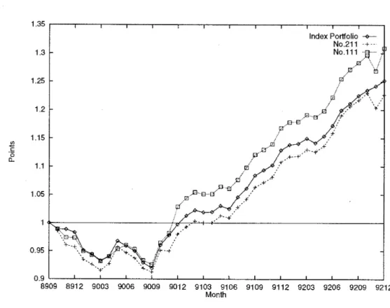
Figure 2 sliows the values of the best and the worst one among these eighty two portfolios in terms of the values at the end of the thirty nine periods horizon. T h e best one labeled No. 211 outperforms the Yamaichi index while the worst one labeled No. I l l is a little behind the index. We see from this figure that we can keep track of the index portfolio very well by using our model. Also Figure 3 shows the monthly rat,es of return of the calculated portfolio and the index portfolio. Let us note that the l~ort~folio consists of at most seven bonds. which is very desirable from the viewpoint of bond managers. Also, the computation time for solving the problem (39) is about 5 seconds on SONY NKS-3800 Workstat ion.

6 Conclusions and t h e Future Direction of Research

We showed in this paper that both partial optimization moclels and tot a1 optimization models proposed in [7] for bond portfolio management of in~tit~utional investors can be solved to optimality in an efficient way by using a global ~pt~imization algorithm developed by one of the authors[9]. In the last several years, a simplified version of the total optimization model has been used by several institutional investors. Instead, a partial optimization model was not used because of computational difficulty. However. it is now ready for use for the first time in a real transaction environment. As st atled in the Introduction, there has been a significant needs of bond managers of institutional investors for a partial optimization model since only a fraction, typically less than one t8enth of the total assets is subject t o transact ion. The partial optimization model meets the request of such bond managers t o evaluate their transaction.

Due to the limited availability of the real market data, we could not conduct an extensive test to fully demonstrate the potential power of this model. Therefore we applied a par- t ial optimization model to t he index t racking of government bonds, by using t he available market clat a. The result shows that this model generates a remarkably good result both in terms of computat,ional efficiency and c~uality of the resulting portfolio. To demonstrate the usefulness of our approach, a more extensive simulation has to be conducted. whose results as well as further improvements of the model will be discussed elsewhere.

Acknowledgements

The first author acknowledges the generous support of the Dai-ichi Life Insurance Co. and the Toyo Trust and Banking Co. Ltd..

(11)

Figure 2: Values of The Port,folios

8912 9003 9006 9009 9012 9103 9106 9109 9112 9203 9206 9209 9212 Month

(12)

References

[l] Avriel.

N..

Nonl-inier Programming. Prent ice-Hall. 1976.

21 Chariies, A. and Cooper. W.W.. m-Programining with Linear Fractional Functions", Naval Research Logistics Quarterly, 9( 1962) 1 8 1 ~ 1 8 6 .

[3] Chvat al. A'. , Linear Programming, Freeman and Co..1983.

[4] Elton. E.J. and Gruber. N.J.. Modem Portfolio Theory and Investment Analysis (4th ed.) John Wiley

fc

Sons. Inc.. 1991.

[5] Fong. G.H. and Fabozzi. F..J.. Fixed Income Portfolio Management. Dow Jones. Invin, Inc., 1985.

[G] Horst, R. and Tuy H., Global Optimization, Springer Verlag. 1991.

71 Konno, H. and Inori, N., "Bond Portfolio Optimization by Bilinear Fractional Pro- gramming". J. of the Operations Research Society of Japan. 32 (1989) 143-158. 8 Ko11110, H. and Talcase, T., "Estimating the Term Structure of Interest Rates by Con-

strained Least Square Approach". to appear in Financial Engineering and Japanese Markets.

[g] Konno, H., Yajima, Y. and Matsui. "Paramet,ric Simplex Algorithms for Solving a Special Class of Nonconvex Minimizat,ion Problems", J. of Global Optinzization, 1 (1991) 65-81.

[l01 Lasdon. L., Opt-in~ization Theory for Large Systems. Macmillian Co., 1970.

[l l] Luenberger. D.G.. Introduction to Linear and Nonlinear Programming. (2nd edit ion). Addison-Wesley. 1984.

Hiroshi KONNO:

Depart,ment of Indust,ria,l Engineering and Mana~gement, Tokyo Inst it,ute of Technology

2-12-1 Oh-olca~a~ma,, Meguro-ku Tokyo 1 52, Japan