A Consistency Improving Method in Binary AHP

Society of Japan

Vol. 38, No. 1, March 1995

A CONSISTENCY IMPROVING METHOD IN BINARY AHP

Kazutomo Nishizawa

Nihon UniVfTsity

(Received March 23, 1992; Final September 2, 1994)

Abstract In this paper, a consistency improving of the comparison matrix in binary AHP (Analytic Hierarchy Process) is studied. As its byproducts, we propose a method to count the cycles oflength 3 and to find the locations of the cycles in a complete directed graph. We apply our proposed consistency improving method to various examples including three actual sports games. Comparing our method with ordinary improving method, we can show the usefulness of our method.

1. Introduction

In the AHP (Analytic Hierarchy Process [1]), the case where an element aij(i

#-

j) of a comparison matrix A takes one of only two intensity scale of importance values [2], either

B

or 1/

B( B

>

1), is called "binary AHP". In general, consistency of a comparison matrix is usually measured by consistency index called "Cl". If Cl

<

0.1, a comparison matrix is consisten t.

In this paper, a consistency improving of a comparison matrix at complete information case in inconsistent binary AHP is studied. In binary case, we can represent A by a directed graph [2] and can evaluate the inconsistency by the number of directed cycles in the graph. It is considered that misjudgments cause cycles in the graph. It is noted that even if we suggest inconsistency in a comparison matrix, decision maker judges collecting ones or not. First we propose a method to calculate the number of cycles in a directed graph through Theorem 1 in §2. Second in §3 we propose a method to locate each cycle. Next, in §4 an algorithm to improve the consistency most effectively by correcting some doubtful judgments is proposed.

In §5, we apply our method to several sports g;ames, which are typical examples of binary AHP. In §6, we compare our method with ordinary improving method.

2. Proposed Criterion of Consistency

In the AHP, consistency of a comparison matrix is usually measured by [1]

(2.1 ) Cl

=

().max-n,)/(n -1)

where

n

is an order of the comparison matrix and), max is its maximum eigen-value. It is said that if the value of Cl is less than 0.1 the comparison matrix is consistent.

The dissatisfadions of Cl that we felt are as follows.

(1) The justification for value 0.1 of Cl is not theoretically clear.

(2) In incomplete information cases, it is impossible to have the value of Cl [3]. Since we want to have consistency before estimating unknown comparisons.

Now we are going to propose a new criterion instead of Cl. We propose our new criterion of consistency for a binary case. This idea is based on graphs and networks. If aij = B then

22 K. Nishizawa

we represent it by a directed arrow (i, j) or i --t j in the corresponding complete graph

in which any two points are connected by an arrow. According to network theory [4], we introduce a vertex matrix

V

whose (i,j) element Vij

=

1(0) if aij

=

0(1/0)

and Vii = O.

The r-th power of the vertex matrix represents the relation connecting r

+

1 points. In the binary case the inconsistency of a comparison matrix is caused by directed cycles in the corresponding graph. It is clear that if there are no cycles in the graph it attains the maximum consistency [2J. Thus we are able to measure the inconsistency by the number of directed cycles (simple cycles hereafter) in the graph. There may be cycles of various lengths, but we have only to consider the cycles of length 3. Because, if we have a cycle 1-2-3-4 of length 4, we are to have a cycle 1-2-4 or 2-3-4 of length 3 according to 2 --t 4

or 4 --t 2.

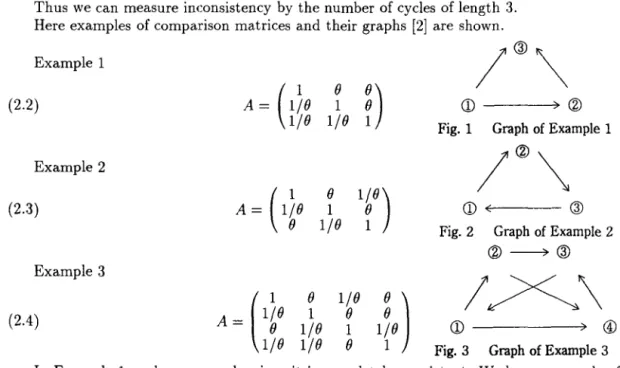
Thus we can measure inconsistency by the number of cycles of length 3. Here examples of comparison matrices and their graphs [2J are shown.

Example 1 (2.2) Example 2 (2.3) Example 3

(2.4)

_A

₌

(I~O

I/O

f

~1)

I/O

o

1

I/O

o

1

I/O

I/O

I/O

o

1

o

CD

)

@

Fig. 1 Graph of Example 1

CD

~(---- @ Fig. 2 Graph of Example 2

@ - > @

I~\

CD

---~)

@

Fig. 3 Graph of Example 3 In Example 1 we have no cycle, since it is completely consistent. We have one cycle of length 3 in Example 2 and two cycles (1-2-3 and 1-4-3) of length 3 in Example 3, since the former has one inconsistency and the latter has two inconsistencies.

In order to find the number of cycles of length 3 we can use the vertex matrix corresponds to the comparison matrix.

In binary case we can easily construct the vertex matrix V from the comparison matrix A as mentioned above. Thus we have the following vertex matrices for Examples 1,2 and 3:

(2.5)

V =

(~ ~

i)

for Example 1,

(2.6) for Example 2,

We can calculate the number of cycles of length 3 in a given complete directed graph, or the inconsistency of a binary comparison matrix, by the following theorem.

Theorem 1 Given a comparison matrix A in the binary AHP, the trace (sum of diagonal elements) of the third power of the vertex matrix V corresponding to A is three times the number of the cycles of length 3; that is,

(2.8)

tr(V 3)/3 =

the number of direct cycles of length 3, where

tr(M)

is the trace of a matrix

M.

n n

Proof The i-th diagonal element of V3 is (V3)ii =

L L

ViaVabVbi where ViaVabVbi == 1 if a=lb=l

and only if points i, a, b, i form a cycle of length 3 (where Vij is

(i,j)

element of V ). Thus

n

(V3

)ii represents the number of cycles that go through point i. Then

L(V3

)ii(=

tr(V3))

i=l represents the number of all cycles counted triple, which states formula (2.8).

Thus our proposed criterion of consistency is judged by diagonal elements of the matrix

V3_{• If diagonal elements of V}3 _{are all 0, this shows the corresponding graph is acyclic and}

we judge it consistent, but if not, the graph is a cyclic and we judge it inconsistent. For Example 1, we have

(2.9)

o

o

0)

0 .

o

0

We see that Fig. 1 is an acyclic graph, since it is consistent. For Example 2, we have

(2.10)

( 1 0

V3 = 0 L

o

0

~)

and

tr(V3)/3

= 1. We see that there is one cycle in Fig. 2. For Example 3, we have

(2.11)

_V 3 ₌

(i

₀

o

and

tr(V3)/3

=

2. We see that the graph in Fig. 3 has two cycles of length 3.

Having found the method to calculate the number of cycles, we proceed to locate each cycle and this serves to improve consistency.

3. Locating of Cycles

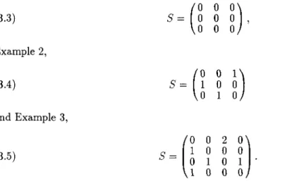
Information on locations of cycles is completely included in the following matrix S;

(3.1 )

where

*

operation means elementwise multiplication of two matrices, that is, for A

24 K. Nishizawa

Theorem 2 Let Sij be (i, j) element of matrix S defined as above then Sij is the number of cycles that includes arc

(i,j)

in the corresponding graph.

n

Proof By definition we have Sij

=

L

ViaVajVji, where "a" runs on all points in the graph.

a=l

If and only if

"a"

satisfies the condition as shown in Fig. 4, that is,

(i,a,j,i)

forms a cycle,

ViaVajVji = 1. Thus Sij is the number of cycles including arc

(i,j).

Of course, we have Sij = 0 if Vji = 0, and Sii = O.

'~la

1 VaJ=l

~

VJI~.

_J

Fig. 4 Condition of fonning a cycle

Therefore if the elements on i-th row of matrix

S

are all zero, point i is not involved in any cycles. If j-th elements on i-th row is n, point i has n arcs on cycles incoming from point j.

Incidentally sum of each i-th row coincides with the value of i-th diagonal element of V3

which represents the number of cycles passing through point i.

Using the information included in matrix S we can find the cycles of length 3 in a given directed graph or a comparison matrix. We make submatrix Sijk composed of elements in the i, j and k-th rows and i, j and k-th columns of matrix S as follows (i, j, k E {I, 2,· .. ,n}, i

<

j

<

k):

(3.2)

If and only if 3 x 3 submatrix Sijk has zero-rows or zero-columns, the point i, j and k form no cycle (where a zero-row means a row whose components are all zeros).

For Example 1, we have

(3.3)

Example 2,

(3.4)

and Example 3,

For Example 3, we have following 4 submatrices,

(~

0

~)

,

S123

=

0 1 forming cycle (D-@-@

(r

0

~)

,

S124

=

0 0 with no cycle,

(~

2

~)

,

S134

=

0 0 forming cycle (D-@-@, and

S234

=

(~

0

~)

0 0 with no cycle.

As a result, we have found two cycles, (D-@-@ and (D-0-@ in Fig. 3.

4. A Consistency Improving Method

Generally speaking, inconsistency in AHP, or the number of cycles in the graph cor-responding to the comparison matrix A, is caused by misjudgments. In our binary case "judge" is the direction of arc in our graph. We often ascertain that reversing the direction of specific arc dissolves many cycles. The direction corresponding such an arc must be based on misjudgment.

If we find (i,j) element with value k in matrix S, we can reduce the number of cycles by

k by reversing the direction of arc (i,j). Roughly speaking, we can reduce the inconsistency by reversing the directions of arcs that have large values in matrix

S.

When there are many such candidates, it is not so clear which arc's direction should be changed most effectively.

Here we show an effective algorithm reducing as many cycles as possible by reversing directions of minimum number of arcs.

Algorithm for extinguishing cycles

Step 1 : Enumerate all cycles of length 3 in the given graph (by the method in §3), and denote the set of all cycles by C.

Step 2 : Enumerate all arcs included in any cycle in C, and denote the set of these arcs by A.

Step 3 : Construct the cycle-arc incidence matrix whose (i,j) element is "I" if i-th cycle in C includes j-th arc in A, and otherwise "0". Or equivalently construct a bipartite graph (C, A;

J)

where

J

is the set of edges connecting e( E

C)

and

a(

E A) are connected by an edge in .J if and only if cycle e includes arc

a.

Step 4 : Find the minimum covering set M(S;; A) which covers all elements of C, where

if a cycle e includes an arc a we say "a covers e". (There are various algorithms to find the minimum covering sets in graph theory.)

Step 5 : Reverse the directions of all arcs in M, then all cycles in the given graph eliminate.

26 K. Nishizawa

For Example 3 (which has Cl = (,,\ max

-n)/(n -

1) = (4.644 - 4)/(4- 1) = 0.215) we have the cycle-arc incidence matrix shown in Table 1.

Table 1 Cycle-arc incidence matrix for Example 3 cycle~arc 0,2) 0,3) 0,4) (2, 3) (3,4)

1-2-3 1 0 1 0

1-3-4

0

1

0

1

The corresponding bipartite graph is shown in Fig. 5.

1-2-3

~

~~:~~

0,4)

1-3-4 (2, 3)

(3, 4) Fig. 5 Bipartite graph for Example 3

We have minimum covering set M = {(I, 3)} as underlined in Fig. 5.

If we reverse the direction of arc (1,3) to (3,1) then all cycles in the graph in Fig. 3 are eliminated and we have Cl = 0.040 reducing the value of Cl by 0.215 - 0.040 = 0.175.

This example shows that our algorithm is useful to suggest the decision maker his mis-judgments. He had thought that

®

is better than

CD,

which resulted a worse consistency,

0.215. If he changed his judgment, that is, if he thought

CD

is better than

®

then it would reduce the value of Cl by 0.175. Thus we can insist that his first decision was a misjudgment. In the following section we treat more detailed examples, sports games that any two teams have a match and one of them wins (and the other loses) with no tie. Let us call such a game "league game". The fact that team i wins (team j loses) corresponds to judgment "i is better than j". Thus league game can be treated as our binary AHP, and our method can be applied to league games.

5. Applications to Sports Games

In order to confirm the validity of our method, we apply our method in AHP to decide ranking in league sports games. In an inconsistent case, cycles of three teams that is triangu-lar contest often occur. It is considered that "misjudgment" in ordinary AHP corresponds to "accidental victory (or defeat)". Our main object is to find out and suggest these accidental results.

Improving consistency corresponds to correcting accidental results. In an inconsistent case the isolated cycle of three teams that is a triangular contest often occurs. Then these three teams are considered to have almost equal ability. Thus we consider there are no accidental results.

5.1 Application 1 (Tokyo six-university baseball league, Fall 1991)

First the Tokyo six-university baseball league is considered. Its results of matches and its graph are shown in Fig. 6 and Fig. 7, respectively. In this case there is only one cycle in Fig. 7.

ill

CID

®

@ _CID @

ill

'"

0

0

0

0

0

CID X

'"

0

X

₀

₀

®

X X

'"

0

0

0

@ X

₀

X

'"

0

0

CID X X X X

'"

0

@

X X X X X ' "

Fig. 6 Results of matches of Application 1 The comparison matrix is shown below.

(5.1 )

I/O

1

A _ I/O l/B

-

I/O

0 [ 1 0

l/B l/B

I/O l/B

o

o

I

I/O

l/B

I/O

o

l/B

B 1

I/O

l/B

ill

- - - - ' ; » CID

i

~

@

@

'\

!

(5)<

®

Fig. 7 "Graph of Application 1

fill

I/O

We obtain A max = 6.390 and Cl = 0.078 where 0

=

2. To find cycles, we have V and S as

below.

V=

[!

1 1 1 1

!l

0 1 0 1 0 0 1 1 1 0 0 1 0 0 0 0 0 0 0 0 (5.2)

(5.3)

s=

[!

0 0 0 0

!l

0 0 1 0 1 0 0 0 0 1 0 0 0 0 0 0 0 0 0 0 Then we find only one cycle as follows.

(5.4)

Thus we judge this case one inconsistency.

We have the cycle-arc incidence matrix in Table 2.

Table 2 Cycle-arc incidence matrix for Application 1

cyc!e"'arc (2.3)(2.4)(3.4)

2-3-4

28 K. Nishizawa

~

(2'3)

2-3-4 (2,4)

(3, 4) Fig. 8 Bipartite graph for Application 1

We have minimum covering set M = {(2,3)} or {(2,4)} or {(3,4)}. Thus we can not suggest inconsistency location in comparison matrix A shown (5.1).

It is just a triangular contest, and we consider that teams @,

CD

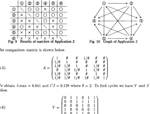
and @ have almost equal ability.

5.2 Application 2 (Private tennis league)

Its results of matches and its graph are shown in Fig. 9 and Fig. 10, respectively. In this case there are three cycles in Fig. 10.

CD

@ @ @ @ @

CD

---~) @

CD

'"

0

0

X

₀

₀

@

x

_"-

₀

₀

₀

₀

i

~

@

x

x

_"-

0

x

₀

@

-@

@

0

x

x

_"-

x

0

@

x

x

₀

₀

_"-

₀

'\

1

@

x

x

x

x

x

),

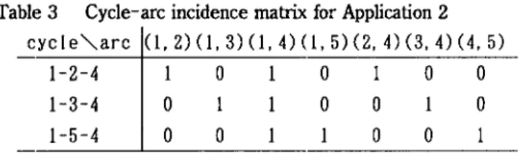
Fig. 9 Results of matches of Application 2 Fig. 10 ~ raph of Application 2 ) @ The comparison matrix is shown below.

[ 1

0 0

I/O

0

!l

I/O

1 0 0 0

(5.5)

A

=

l~O

I/O

1 0 1/()

I/O I/O

1

I/O

I/O I/O

0 0 1

I/O I/O I/O

l()

_I/O

We obtain). max = 6.641 and Cl = 0.128 where 0 = 2. To find cycles we have V and S as below. 0 1 1 0 1 1 0 0 1 1 1 1 (5.6) V= 0 0 0 1 0 1 1 0 0 0 0 1 0 0 1 1 0 1 0 0 0 0 0 0

s=

[I

0 0 3 0

11

0 0 0 0 (5.7) 0 0 0 0 1 1 0 1 0 0 0 0 0 0 0 0

Then we find three cycles as follows.

(5.8)

(5.9)

(5.10)

Thus we judge this case three inconsistencies. We have the cycle-arc incidence matrix in Table 3.

Table 3 Cycle-arc incidence matrix for Application 2 cyc(e"'-arc 0,2) 0,3) 0,4) 0,5) (2,4) (3,4) (4, 5) 1-2-4 1-3-4 1-5-4

o

o

o

1

o

o

o

o

o

o

1

o

The corresponding bipartite graph is shown in Fig. 11.

1-2-4 1-3-4 1-5-4 ___ 0,2)

~

0,3) ~

0,

5) ~ (2,4) ~ (3,4) - - - (4,5) Fig. 11 Bipartite graph for Application 2

o

o

1

We have M = {(1,4)} as underlined in Fig. 11. Thus we suggest that inconsistency location in comparison matrix A, (5.5), is a14.

If we reverse the direction of arc (4,1) to (1,4) then all cycles in Fig. 10 are eliminated and we have Cl = 0.054.

We consider that team

®

won an accidental victory over team

CD.

5.3 Application 3 (East-metropolis universities baseball league, Fall 1991) Its results of matches and its graph are shown in Fig. 12 and Fig. 13, respectively. In this case there are four cycles in Fig. 13.

30 K. Nishizawa

CD

<ID

@ @) @ @

CD

---~)

<ID

CD

_"-

0

0

0

0

0

<ID

x

_"-

x

₀

₀

₀

i

~

@ X

₀

_"-

X X

₀

@

@

@) X X

₀

_"-

₀

X @ X X

₀

X

_"-

₀

\:

7

X

@

x

x

x

0

"-Fig. 12 Results of matches of Application 3 Fig. 13 Graph of ApplicatIOn 3 @<

@

The comparison matrix is shown below.

[ 1 () () () ()

n

1/() 1 1/() () () (5.11 )

_A

₌₌ 1/()

_{I/O I/O}

() 1 1/() 1/() 0 1 0

I/O I/O

0 1/() 1 1/() 1/() 1/() 0 1/()

We obtain Amax

=

6.744 and Cl

=

0.149 where 0

=

2. To find cycles we have V and S as below.

V~

[!

0 0 1 1 1 1 1 1

₁₁

(5.12) 1 0 0 0 0 1 0 1 0 1 0 0 0 0 1 0

S~

[I

0 0 0 0

!l

0 2 0 0 (5.13) 0 0 2 1 1 0 0 0 1 0 1 0 0 1 0 1 Then we find four cycles as follows.

S234

=

(~

2

~)

(5.14) ₀ 0 S235

=

(~

2

~)

(5.15) 0 0 S346

=

(~

2

~)

(5.16) 0 0 S456

=

(~

0

~)

(5.17) ₀ 1

Thus we judge t.his case four inconsistencies. We have the cycle-arc incidence matrix in Table 4.

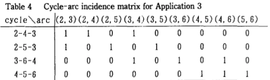
Table 4 Cycle-arc incidence matrix for Application 3

cyc!e""-arc

(2,3) (2,4) (2,5) (3,4) (3,5) (3,6) (4,5) (4,6) (5,6)

2-4-3 0 0 0

2-5-3 0 0

1

0

3-{j-4 0 0 0 0

4-!i-6 0 0 0 0 0 0

The corresponding bipartite graph is shown in Fig. 14.

2-4-3

Lfh1l

(2, 4)

2

(2. 5) 2-5-3 (3, 4) (3, 5) 3-6-4 (3,6) 4-5-6

::s::

(4, 5) ~ - - (5.6) Fig. 14 Bipartite graph for Application 3

0 0 0

0 0 0

0 0

We have M = {(2, 3), (4, 6)} as underlined in Fig. 14. Thus we suggest that inconsistency locations in comparison matrix A, (5.11), are a2:l and a46.

If we reverse the direction of arc (3,2) to (2,3) and arc (6,4) to (4,6) then all cycles in Fig. 13 are eliminated and we have Cl = 0.054.

In this case, we have three candidates (2,3), (3,4) and (4,6), include two cycles in Table 4. Rewriting these candidates, of course, all cycles are eliminated. In Fig. 14, we see that it is not always necessary to rewriting all candidates.

6. Comparison of Our Improving Method with Ordinary One

The ordinary or conventional consistency improving method [5], is (a) to find the maxi-mum error element, (b) to correct it and (c) to calculate the new eigen-vector 101,' .. ,Wn of

the corrected comparison matrix. In this method an error calculation is based on (6.1).

(6.1 )

[eij]

=1

(aij - w;/1Oj)

1

However, estimating inconsistency, here, rela,tive error (6.2) instead of (6.1) was calcu-lated.

(6.2)

For Application 3, we have A max = 6.744, Cl = 0.149 and the following eigen-vector

W, which are normalized with sum of elements equal to 1 (0 = 2).

32 K. Nishizawa

First, using (6.2), for comparison matrix A, (5.11), we have

(6.4) [ 0.000 0.279 0.145 0.145 0.386 0.000 1.370 0.408 [ _{e'J -}.. ] _ 0.170 0.578 0.000 1.000 _{0.170 0.688 0.500 0.000} 0.118 0.613 0.522 0.911 0.099 0.300 0.541 0.615 0.105 0.110) 0.380 0.231 1.093 0.351 0.477 1.596 . 0.000 0.380 0.613 0.000

The maximum element of (6.4) is e46 (as underlined). We correct a46 from liB to B (a64

from B to liB) and estimate again, we have

(6.5) [ 0.000 0.273 0.110 0.376 0.000 1.449 0.124 0.592 0.000

[eij]

= 0.326 0.927 0.410 0.061 0.542 0.528 0.375 0.092 0.112 0.246 0.058 0.601) 0.481 0.352 0.101 0.696 1.119 0.100 0.000 0.375 0.061 ' 0.601 0.000 0.151 0.058 0.178 0.000

.A max

=

6.512 and Cl = 0.102. The maximum element of (6.5) is e23 (as underlined). We

correct a23 from liB to B (a32 from B to liB) and estimate again, we have

(6.6) [ .. ] _ 0.206 0.000 0.000 0.260 0.587 0.370 [ 0.000 0.370 0.260 0.206 0.000 0.587) 0.587 0.000 0.000 0.370 0.206 0.260 e'J - 0.260 0.587 0.206 0.000 0.370 0.000 ' 0.000 0.260 0.370 0.587 0.000 0.206 0.370 0.206 0.587 0.000 0.260 0.000

.A max

=

6.271 and Cl

=

0.054. The maximum element of (6.6) is e16 (as underlined). We correct a16 from B to liB (a61 from liB to B) and estimate again, we have

(6.7) [ .. ] _ 0.032 0.052 0.000 0.303 0.614 0.585 [ 0.000 0.456 0.034 0.327 0.166 2.429) 0.839 0.000 0.050 0.381 0.233 0.212 el ) - 0.485 0.614 0.233 0.000 0.381 0.364 ' 0.199 0.303 0.381 0.614 0.000 0.486 0.708 0.268 1.411 0.571 0.947 0.000

.A max = 6.782 and Cl = 0.156, thus we have a worse result than (6.6), since stop the iteration and (6.6) can be considered as a final result. This coincides with our result mentioned in

§ 5.3.

By ordinary method they must have much larger calculation. Further, according to our method, we can easily suggest to correct a23 and a46 at the same time with very small calculation. If comparison matrix size becomes larger and has a lot of cycles, our method must be very effective.

7. Conclusion

To measure inconsistency of comparison matrix in binary AHP, we proposed a new crite-rion to count how many cycles in its graph. Further, we developed a consistency improving method, by finding and removing cycles in the graph. Our algorithm eliminates cycles in a graph most effectively. We have applied our proposed consistency improving method to various examples including three actual sports games. Comparing our method with ordinary improving method, we can show the usefulness of our method.

Acknowledgments

The author wishes to thank Dr. Iwaro Takahashi, Professor of Nihon University, for useful advice on this investigation. The author is grateful to the referees for their valuable and helpful comments.

References

[IJ

Saaty, T. L. : A Scaling Method for Priorities Hierarchical Structures, J. of Mathematical Psychology, Vol. 15, (1977), 234-281.

[2] Takahashi, I: AHP Applied to Binary and Ternary Comparisons, J. of O. R. Society of

Japan, Vol. 33, (1990), 199-206.

[3] Takahashi, I and M. Fukuda: Comparisons of AHP with other methods in binary paired comparisons, Proceedings of the Second Conference of the Association of Asian-Pacific Operational Research Societies within IFORS, (1991), 325-331.

[4] Busacker, R. G. and T. L. Saaty: Finite Graphs and Networks: An Introduction with Applications (in Japanese), Baifu-kan, (1981), 199-200.

[5] Tone, K : Gemu kankaku ishi-kettei-hou : Introduction to the AHP (in Japanese), Nikka-giren, (1990), 38-40.

Kazutomo :~ishizawa

Department of Mathematical Engineering,

College of Industrial Technology, Nihon University, 1-2-1, Izumicho, Narashino, Chiba, 275, Japan e-mail: [email protected]