Resultant-factorization Technique for Obtaining Solutions to Ordinary Differential Equations

全文

(1)Vol.2011-MPS-84 No.9 2011/7/18 IPSJ SIG Technical Report. and variables render, the computational cost of Gröbner basis increases. This leads us to propose a resultant-factorization technique1) that provides the desired irreducible affine variety (solution). By using the resultant-factorization technique, we can reduce the computational cost of Gröbner basis.. Resultant-factorization Technique for Obtaining Solutions to Ordinary Differential Equations Kinji Kimura. †1. and Hiroshi Yoshida. 2. Resultant-factorization technique. †2. On the basis of6) , we propose an efficient technique to arrive at the targeted affine variety (solution); the technique is shown in Fig. 1(a). Let BP = {BPi |1 ≤ i ≤ n} be an original set of polynomials. Let F1 be a set of n−1 resultants of polynomials BPj (1 ≤ j ≤ n, i 6= j) for some BPi (1 ≤ i ≤ n) in a variable, say, x1 . It is reasonable to select a variable x1 such that BPi and BPj are low-degree polynomials in x1 . For instance, if one can factorize some element f in F1 into mutually disjoint elements f1 , f2 , and f3 , hF1 i can be decomposed into hF1 , f1 i ∩ hF1 , f2 i ∩ hF1 , f3 i. As a result of the factorization, the resultant F21 in x2 can usually be described by a smaller set of polynomials. Furthermore, when one obtains a factorized term like (y1 + y22 )(z − y32 + 3)3 with the rate constants y1 and y2 , it is sufficient to consider only (z − y32 + 3) because the rate 2 constants are √ guaranteed to be positive (y1 > 0 ∧ y2 > 0 ⇒ y1 + y2 > 0) and the radical hBP i suffices. We can also ignore a factor like (y1 − y2 ) when we assume y1 6= y2 because of unacceptable factors or mathematically trival factors. These simplifications allow us to prune the branches of the resultant-factorization series?1 . When we arrive at an appropriate ideal (hF32 i in Fig. 1(a)), we can efficiently determine all the rate constants by using the ideal hBP i + hF32 i, as illustrated in Fig. 1(a).. We propose a technique for obtaining solutions to ordinary differential equations. A system of differential equations sometimes has multiple solutions with distinct features. Prime ideal decomposition can be used for extracting the desired solution from these solutions. Solutions to algebraic equations contain many parameters, and in such a case, prime ideal decomposition is less tractable. As an alternative, we propose a resultant-factorization technique for extracting the desired solution. We also demonstrate the implementation of this technique and show its timing data.. 1. Introduction In ordinary differential equations, we often need to analyze complicated polynomials with multiple irreducible affine varieties (solutions). It is therefore essential to perform prime ideal decomposition. To understand the importance of the decomposition, consider the following set of polynomials: {x3 − x2 y − xy − 2x + y 2 + 2y, xy −x−y 2 +y}. Prime ideal decomposition shows that the above polynomials can be decomposed into two irreducible affine varieties, {x−y} and {x2 −3, y−1}. While one cannot determine concrete values of x and y using the former, one can √ determine them, x = ± 3 and y = 1, using the latter. Hence, to decide whether or not we can determine the values of variables, we must perform prime ideal decomposition of polynomials. In ordinary differential equations, however, there are many parameters and variables that describe observed data and systems, respectively. In general, large numbers of parameters and variables render prime ideal decomposition more difficult4) . Especially, the method in4) needs the computation of Gröbner basis in the beginning. Under large numbers of parameters. 3. Implementation We have implemented our “Resultant-factorization technique,” which is shown as “ScodeRFP.rr” on http://sites.google.com/site/codes86/. The main routine of “ScodeRFP.rr” is “automatic decom,” which calls the following seven procedures: ( 1 ) Procedure 1: shortcut speed(ideal I, list of polynomials lp) returns an ideal. †1 Kyoto University †2 Kyushu University. ?1 Recently, such a pruning procedure in algebraic approaches has been studied, e.g., “positive quantifier elimination”(QE)5) .. 1. c 2011 Information Processing Society of Japan °.

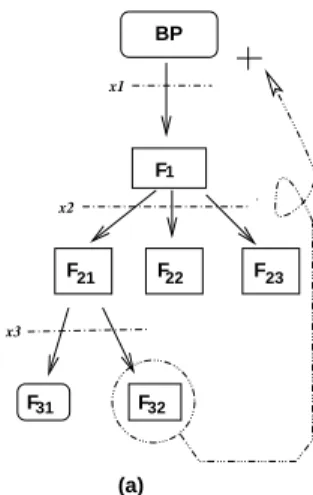
(2) Vol.2011-MPS-84 No.9 2011/7/18 IPSJ SIG Technical Report. to calculate resultants in the next procedure because the resultant of polynomials p and q in x is q r , where q does not contain the variable x and r is the degree of x in p. ( b ) Otherwise, we select a variable as follows: ( i ) We calculate di – the maximum degree of variable xi (1 ≤ i ≤ n) by considering lp. If a single dj is the minimum among di (1 ≤ i ≤ n), xj is returned. ( ii ) If multiple di ’s have the same minimum value, let y1 , y2 , . . . , ym be variables that provide this minimum. We calculate ni , the number of polynomials that contain yi . If a single nj provides the minimum among ni (1 ≤ i ≤ m), yj is returned. ( iii ) If multiple ni ’s provide the same minimum, let z1 , z2 , . . . , zk be the variables that provide this minimum. We calculate ti which means the number of terms in the polynomials that contain zi . Variable zj that provides the minimum and that is calculated first is returned. In (i)-(iii), as an accompanying output, we return the polynomial that contains the returned variable and has the minimum number of terms. ( 7 ) Procedure 7: idealresultant returns a set of resultants on the basis of the output of Procedure 6. We perform Procedures 1,2,. . . ,7 for a given input ideal. Procedure 5 gives rise to branches of Procedures where the main routine is recursively called. Finally, the main routine returns a list of polynomials together with the input original ideal. Prime ideal decomposition can be rapidly performed for each of the polynomials in the list.. BP x1. F1 x2. F21. F22. F23. x3. F31. F32. (a). Fig. 1 Schematic illustration of the resultant-factorization technique. (2) (3) (4). (5). (6). obtained by removing the factors in lp from ideal I. This procedure aims to remove unacceptable factors or mathematically trival factors. Procedure 2: idealclean(ideal I) returns an ideal obtained by removing redundant elements from ideal I. Procedure 3: coefficientcleaner(ideal I, poly p) returns an ideal obtained by removing common factors and p from ideal I. Procedure 4: constant check(ideal I) checks whether or not ideal I has an element composed of only the parameters. If there is such an element , the function returns 0 to indicate the presence of an error in the top-level function. Procedure 5: idealfactorize returns a list of elements that can be factorized over Q in a given ideal; if there are no such elements in the ideal, then √ it returns the given ideal. This is based on the relation < I, f ∗ g > = √ √ < I, f > ∩ < I, g >. Procedure 6: variable choice returns a variable that is to be removed in the next procedure. There are two types of outputs. Let lp be a given list of polynomials. ( a ) In lp, when there is a variable contained in only one polynomial, “variable choice” returns the variable. In this case, it is not necessary. 4. Model In this section, we introduce the Painlevé VI equation2) ( ) ( ) 1 1 1 1 1 1 1 2 y 00 = + + y0 − + + y0 2 y y−1 y−t t t−1 y−t ( 2 ) α1 α42 t y(y − 1)(y − t) α32 (t − 1) α02 − 1 t(t − 1) + × − + − , t2 (t − 1)2 2 2 y2 2 (y − 1)2 2 (y − t)2. 2. (1). c 2011 Information Processing Society of Japan °.

(3) Vol.2011-MPS-84 No.9 2011/7/18 IPSJ SIG Technical Report. which is an ordinary differential equation. Painlevé VI equation (1) has four parameters:α0 , α1 , α3 , and α4 . We discuss typical solutions, which are called “rational solutions.” All rational solutions for the equation have been obtained in3) . We can use algebraic geometry for studying the equation (1). However, in general, we cannot use these techniques for all ordinary differential equations. Thus, we treat equation (1) in the condition that we do not know the mathematical structure of the equation (1). We assume rational solutions of the form y(t) = (k0 + k1 t + k2 t2 )/(l0 + t) and substitute these solutions in the equation. We then obtain algebraic equations for the eight variables k0 , k1 , k2 , l0 , α0 , α1 , α3 , and α4 . By using the resultant-factorization technique proposed in the previous section 2, we can determine the solutions. We assume rational solutions of the form y(t) = (k0 + k1 t + k2 t2 )/(l0 + t) and substitute these solutions in the equation (1). Then, we get the following ideal, P = {−k04 × (α1 k0 + (−α1 − α3 )l0 ) × (α1 k0 + (−α1 + α3 )l0 ), . . . , −k24 × (α1 k2 − α1 + α0 ) × (α1 k2 − α1 − α0 )} = {p1 , p2 , . . . , p13 } = 0. (2) For convenience, we define five equations: f1 = α1 k0 + (−α1 + α3 )l0 , f2 = α1 k0 + (−α1 − α3 )l0 , g1 = α1 k2 − α1 + α0 , g2 = α1 k2 − α1 − α0 , and h = k0 − l0 k1 + l02 k2 . Hence, we can divide the original problem(P = 0) to the six cases, P1 = {f1 , p2 , · · · , p12 , g1 } = 0, P2 = {f1 , p2 , · · · , p12 , g2 } = 0, P3 = {f2 , p2 , · · · , p12 , g1 } = 0, P4 = {f2 , p2 , · · · , p12 , g2 } = 0, P5 = {k0 , p2 , · · · , p12 , p13 } = 0, P6 = {p1 , p2 , · · · , p12 , k2 } = 0.. ( 2 ) Step 2: we compute, (0). (0). We factorize R2. (1). (0). S2. (0). (1). (0). T3. (0). (1). (1). (1). (0). (1). (1). (0). (1). (1). (1). (1). (0). (1). (0). T3. (0). T4. Q12 . k2 − 1. (1). = resultantα1 (S2 , S3 ), . . . , T11 = resultantα1 (S2 , S11 ). (0). (0) T11 (1). R2 (1) (0) (1) (0) , R = R3 , . . . , R12 = R12 . l0 (k0 − l0 ) 3. (0). (1). (1). We factorize T2 , · · · , T11 and set T3 , . . . , T11 ,. (1) (1) Q1 , . . . , Q12 , (0). (1). = resultantα4 (R12 , R2 ), . . . , S11 = resultantα4 (R12 , R11 ). (0). (0). (1). (1). We factorize S2 , · · · , S11 and set S2 , . . . , S11 , √ √ (0) (0) ( )2 ( )2 S S3 (0) (1) (1) (0) (1) (1) 4 2 S = l S , S = , S2 = 4l04 S2 , S2 = 0 3 2 4l04 3 l04 ··· √ (0) ( )2 ( )2 S10 (0) (1) (1) (0) (1) 4 2 S10 = l04 S10 S = l (k − 1) , S2 = , S , 0 2 11 11 l04 √ (0) S11 (1) S2 = 4 l0 (k2 − 1)2 ( 4 ) Step 4: we compute,. (0). Q1 = Q1 , . . . , Q11 = Q11 , Q12 = (k2 − 1)Q12 , Q12 =. (1). ( 3 ) Step 3: we compute,. (0). and set. (1). (0). (1). (. (1). = l06 (k2 − 1)2 (k0 − l0 )2 h2 T3. )2. ( )2 (1) (1) = l04 (k2 − 1)2 h2 T4 , T4 =. Q12 = resultantα0 (g1 , p12 ). We factorize. (0). and set R2 , . . . , R12 ,. (0). Q1 = resultantα0 (g1 , f1 ), Q2 = resultantα0 (g1 , p2 ), . . . (0) Q12. (1). R2 = l0 (k0 − l0 )R2 , R2 =. We explain the resultant-factorization technique for the case of P1 = 0 in detail. Thus, we consider the ideal, < f1 , p2 , · · · , p12 , g1 > . We compute solutions in the case of f1 = 0 and g1 = 0 as follows, ( 1 ) Step 1: we compute, (0). (1). R2 = resultantα3 (Q1 , Q2 ), . . . , R12 = resultantα3 (Q1 , Q12 ).. = l04 (k2 − 1)2 h2. (. (1) T11. )2. √ (1) , T11. =. (1). , T3 √. √. =. (0). T3 6 l0 (k2 − 1)2 (k0 − l0 )2 h2. (0). T4 ,··· , l04 (k2 − 1)2 h2 (0). T11 . l04 (k2 − 1)2 h2. ( 5 ) Step 5: from the process of the above-mentioned computation, we can assume the following conditions, k2 6= 1, l0 6= 0, k0 6= l0 , h 6= 0, k0 6= 0.. 3. c 2011 Information Processing Society of Japan °.

(4) Vol.2011-MPS-84 No.9 2011/7/18 IPSJ SIG Technical Report. ( 6 ) Step 6: we compute the Gr¨ obner basis(G0 )4) of the ideal, < (1) (1) T3 , · · · , T11 > . ( 7 ) Step 7: by using saturation technique4) , we remove the component k2 − 1 from the ideal(G0 ), G1 =< G0 , 1 − u(k2 − 1) > . ( 8 ) Step 8: by using saturation technique, we remove the component l0 from the ideal(G1 ), G2 =< G1 , 1 − u(l0 ) > . ( 9 ) Step 9: by using saturation technique, we remove the component k0 − l0 from the ideal(G2 ), G3 =< G2 , 1 − u(k0 − l0 ) > . ( 10 ) Step 10: by using saturation technique, we remove the component h from the ideal(G3 ), G4 =< G3 , 1 − u(h) > . ( 11 ) Step 11: by using saturation technique, we remove the component k0 from the ideal(G3 ), G5 =< G4 , 1 − u(k0 ) > . ( 12 ) Step 12: we can get the ideal(G6 ) by using computation of the following ideal, G6 =< G5 , P1 > . ( 13 ) Step 13: we get solutions(D1 ) from G6 by using prime ideal decomposition.. Table 1 computing Cases f1 = 0 & g1 = 0 f1 = 0 & g2 = 0 f2 = 0 & g1 = 0 f2 = 0 & g2 = 0. time for different cases Time Solutions 4m34s D1 4m46s D2 4m35s D3 4m41s D4. Cases k0 = 0 l0 = 0 k2 = 0. Time 351m56s 45s 146m14s. Solutions D5 D6 D7. Cases k2 = 1 k0 = l0 h=0. Time 7s 78m57s 3s. Solutions D8 D9 D10. D1 = {{α1 + 2, k1 + 2k2 + α4 , −k1 + α3 + 1, 2k2 − α0 − 2, −k1 + 2l0 k2 − l0 , −2k0 + l0 k1 + l0 , (−4k2 + 2)k0 + k12 + k1 }, · · · {k1 + 2k2 − 2, k0 − k2 − l0 + 1, α4 + 2, α1 − α3 − α0 + 1, α3 l0 − α1 + α3 − 1, −α1 k2 + α3 − 1}, · · · } = 0 D5 = {{l0 , k2 , −α3 + α4 + α1 , α0 + 1, −α4 − k1α1 }, · · · {l0 , k1 + k2 − 1, α4 + 1, α0 + α3 + α1 , α3 + k2 α1 }, · · · {l0 , α1 + 1, α4 + k1 + k2 , α3 + k1 − 1, α0 + k2 − 1}, · · · {l0 , k2 , k1 − 1, α3 }, {k2 , k1 − l0 − 1, α1 + 1, −α0 + α3 + α4 , (l0 + 1)α3 + l0 α4 }, · · · {k2 , α4 + 1, α0 + α3 + α1 + 2, (l0 + 1)α3 + α1 + l0 + 1, k1α1 + l0 + 1, k1α3 + k1 − 1}, · · · {k2 , k1 − l0 − 1, α1 − 1, −α0 + α3 + α4 , (l0 + 1)α3 + l0 α4 }, · · · {k2 , α4 + 1, −α0 − α3 + α1 − 2, (l0 + 1)α3 − α1 + l0 + 1, k1α1 − l0 − 1, k1α3 + k1 − 1}, · · · {k1 − l0 k2 , α3 + 1, α0 − α4 + α1 , −α4 + k2 α1 }, · · · {k1 + k2 − l0 − 1, −α3 + α4 − α1 + 2, α0 + 1,. 5. Timing data If we do not use the resultant-factorization technique, we cannot obtain all the solutions for the ideal (2) within 48 h. However, we can compute solutions with Table 1 by using the resultant-factorization technique. Since the solutions of the equation (1) has a large number of irreducible affine varieties, the resultantfactorization technique functions effectively. Table 1 shows the computing times for the different cases. All the algorithms are implemented on Risa/Asir ?1 and measurements are performed on a PC with Intel Core i7 920 and 12 GB of main memory. 6. Solutions We show D1 , D5 , D6 , D7 , D8 , D9 and D10 .. ?1 http://www.math.kobe-u.ac.jp/Asir/asir.html. 4. c 2011 Information Processing Society of Japan °.

(5) Vol.2011-MPS-84 No.9 2011/7/18 IPSJ SIG Technical Report. −α4 − l0 α1 − 1, (k2 − 1)α1 + 1, (−k2 + 1)α4 − k2 + l0 + 1}, · · · {k1 + 1, α3 + 2, α0 − α4 + α1 + 1, l0 α4 + α1 + 1, −α4 + k2 α1 + 1}, · · · {k1 − l0 k2 , α3 + 1, −α0 + α4 + α1 , −α4 − k2 α1 }, · · · {k1 + k2 − l0 − 1, −α3 − α4 − α1 + 2, α0 − 1, α4 − l0 α1 − 1, (k2 − 1)α1 + 1, (k2 − 1)α4 − k2 + l0 + 1}, · · · {k1 + 1, α3 + 2, −α0 + α4 + α1 + 1, −l0 α4 + α1 + 1, −α4 − k2 α1 − 1}, · · · {k2 , k1 − l0 − 1, α1 + 1, α0 + α3 + α4 , (l0 + 1)α3 + l0 α4 }, · · · {k2 , α4 + 1, −α0 + α3 + α1 + 2, (l0 + 1)α3 + α1 + l0 + 1, k1α1 + l0 + 1, k1α3 + k1 − 1}, · · · {k2 , k1 − l0 − 1, α1 − 1, α0 + α3 + α4 , (l0 + 1)α3 + l0 α4 }, · · · {k2 , α4 + 1, α0 − α3 + α1 − 2, (l0 + 1)α3 − α1 + l0 + 1, k1α1 − l0 − 1, k1α3 + k1 − 1}, · · · , {k2 , k1, α4 }, {k1 − l0 k2 , α3 + 1, α0 + α4 + α1 , α4 + k2 α1 }, · · · {k1 + k2 − l0 − 1, −α3 − α4 − α1 + 2, α0 + 1, α4 − l0 α1 − 1, (k2 − 1)α1 + 1, (k2 − 1)α4 − k2 + l0 + 1}, · · · {k1 + 1, α3 + 2, α0 + α4 + α1 + 1, −l0 α4 + α1 + 1, α4 + k2 α1 + 1}, · · · {k1 − l0 k2 , α3 + 1, −α0 − α4 + α1 , α4 − k2 α1 }, · · · {k1 + k2 − l0 − 1, −α3 + α4 − α1 + 2, α0 − 1, −α4 − l0 α1 − 1, (k2 − 1)α1 + 1, (−k2 + 1)α4 − k2 + l0 + 1}, · · · , {k2 − 1, k1 − l0 , α0 }, {k1 + 1, α3 + 2, −α0 − α4 + α1 + 1, l0 α4 + α1 + 1, α4 − k2 α1 − 1}, · · · } = 0. D7 = {{k0 , α4 + 1, α1 + α3 + α0 + 2, (α3 + 1)l0 + α1 + α3 + 1, α1 k1 + l0 + 1, (α3 + 1)k1 − 1}, · · · {k1 − l0 − 1, k0 , α1 + 1, α4 − α3 + α0 , (α4 − α3 )l0 − α3 }, · · · {k0 , α4 + 1, α1 − α3 + α0 + 2, (α3 − 1)l0 − α1 + α3 − 1, α1 k1 + l0 + 1, (α3 − 1)k1 + 1}, · · · {k1 − l0 − 1, k0 , α1 + 1, α4 + α3 + α0 , (α4 + α3 )l0 + α3 }, · · · {k1 , k0 , α4 }, {k0 − l0 k1 , α1 − α4 + α3 , α0 + 1, α1 k1 − α4 }, · · · {k0 + k1 − l0 − 1, α3 − 1, α1 − α4 + α0 + 2, (α4 − 1)l0 + α1 , α1 k1 + l0 − α1 , (α4 − 1)k1 − α4 }, · · · {k1 + l0 , −α1 + α4 − α3 − 1, α0 + 2, (−α1 − 1)l0 − α4 , −α1 k0 + (α4 − 1)l0 , (−l0 − α4 )k0 + (−α4 + 1)l02 }, · · · {k1 + l0 , −α1 + α4 − α3 + 1, α0 + 2, (−α1 + 1)l0 − α4 , −α1 k0 + (α4 + 1)l0 , (l0 − α4 )k0 + (−α4 − 1)l02 }, · · · {k0 − l0 k1 , α1 + α4 + α3 , α0 + 1, α1 k1 + α4 }, · · · {k0 + k1 − l0 − 1, α3 − 1, α1 + α4 + α0 + 2, (α4 + 1)l0 − α1 , α1 k1 + l0 − α1 , (α4 + 1)k1 − α4 }, · · · {k1 + l0 , −α1 − α4 − α3 − 1, α0 + 2, (−α1 − 1)l0 + α4 , −α1 k0 + (−α4 − 1)l0 , (−l0 + α4 )k0 + (α4 + 1)l02 }, · · · {k1 + l0 , −α1 − α4 − α3 + 1, α0 + 2, (−α1 + 1)l0 + α4 , −α1 k0 + (−α4 + 1)l0 , (l0 + α4 )k0 + (α4 − 1)l02 }, · · · {k0 − l0 k1 , α1 + α4 − α3 , α0 + 1, −α1 k1 − α4 }, · · · {k0 + k1 − l0 − 1, α3 + 1, α1 + α4 + α0 + 2, (α4 + 1)l0 − α1 , α1 k1 + l0 − α1 , (α4 + 1)k1 − α4 }, · · · {k1 + l0 , −α1 − α4 + α3 − 1, α0 + 2, (α1 + 1)l0 − α4 , α1 k0 + (α4 + 1)l0 , (−l0 + α4 )k0 + (α4 + 1)l02 }, · · · {k1 + l0 , −α1 − α4 + α3 + 1, α0 + 2, (α1 − 1)l0 − α4 , α1 k0 + (α4 − 1)l0 , (l0 + α4 )k0 + (α4 − 1)l02 }, · · · {k0 − l0 k1 , α1 − α4 − α3 , α0 + 1, −α1 k1 + α4 }, · · · {k0 + k1 − l0 − 1, α3 + 1, α1 − α4 + α0 + 2, (α4 − 1)l0 + α1 , α1 k1 + l0 − α1 , (α4 − 1)k1 − α4 }, · · · {k1 − 1, k0 − l0 , α3 }, {k1 + l0 , −α1 + α4 + α3 − 1, α0 + 2, (α1 + 1)l0 + α4 , α1 k0 + (−α4 + 1)l0 , (−l0 − α4 )k0 + (−α4 + 1)l02 }, · · · } = 0. D6 = {{k2 , k0 + k1 − 1, α1 , α3 + 1, α4 + α0 + 2, (α4 + 1)k1 − α4 }, · · · {k1 + 2k2 − 2, k0 − k2 + 1, α1 , α4 + 2, α3 + 1, α0 }, · · · {k1 + k2 − 1, k0 , α4 + 1, α1 + α3 + α0 , α1 k2 + α3 }, · · · {k2 , k0 , α1 + α4 − α3 , α0 + 1, −α1 k1 − α4 }, · · · {k0 , α1 + 1, k1 + k2 + α4 , k1 − α3 − 1, k2 + α0 − 1}, · · · {k1 + k2 − 1, k0 , α4 + 1, α1 + α3 − α0 , −α1 k2 − α3 }, · · · {k1 , k0 , α3 + 1, α1 + α4 + α0 , α1 k2 + α4 }, · · · {k1 , k0 , α3 + 1, α1 + α4 − α0 , −α1 k2 − α4 }, · · · {k2 , k1 , α1 , α4 , α3 + 1, α0 + 2}, · · · , {k2 , k1 − 1, k0 , α3 }, {k2 , k1 , k0 , α4 }, {k2 − 1, k1 , k0 , α0 }} = 0. 5. c 2011 Information Processing Society of Japan °.

(6) Vol.2011-MPS-84 No.9 2011/7/18 IPSJ SIG Technical Report. D8 = {{k1 + 1, k0 , α1 + 1, α4 , α3 + 2, α0 }, · · · , {k1 − l0 , k0 , α0 }, {k0 − l0 k1 + l02 , α1 + 1, k1 − l0 + α4 + 1, k1 − l0 + α3 − 1, α0 }, · · · {k1 − l0 , 2k0 − l02 − l0 , α1 + 2, l0 + α4 + 2, l0 + α3 − 1, α0 }, · · · {k0 − l0 k1 + l02 , α1 + 1, k1 − l0 + α4 + 1, k1 − l0 − α3 − 1, α0 }, · · · {k1 − l0 , 2k0 − l02 − l0 , α1 + 2, l0 + α4 + 2, l0 − α3 − 1, α0 }, · · · {k1 , k0 − l0 , α1 + 1, α4 + 2, α3 , α0 }, · · · } = 0. References 1) H. Yoshida, K. Kimura, N. Yoshida, J. Tanaka, and Y. Miwa: Algebraic approaches to underdetermined experiments in biology, Vol.3, pp.62–69 (2010). 2) K. Kajiwara, T. Masude, M. Noumi, Y. Ohta, and Y. Yamada: Determinant formulas for the Toda and discrete Toda equations, Funkcial. Ekvac., Vol.44, pp.291–307 (2001). 3) M. Mazzocco: Rational solutions of the Painlevé VI equation, J. Phys. A: Math. Gen., Vol.34, pp.2281–2294 (2001). 4) T. Shimoyama and K. Yokoyama: Localization and primary decomposition of polynomial ideals, J. Symbolic Comput., Vol.22(3), pp.247–277 (1996). 5) T. Sturm and A. Weber: Investigating genetic methods to solve Hopf bifurcation problems in algebraic biology, Algebraic Biology (K.Horimoto, G. Regensburger, M. Rosenkranz, and H.Yoshida, ed.), Lecture Notes in Computer Science, Vol.5147, Springer(Heidelberg), pp.200–215 (2008). 6) Y. Kawano, K. Kimura, H. Sekigawa, M. Noro, K. Shirayanagi, M. Kitagawa, and M. Ozawa: Existence of the exact CNOT on a quantum computer with the exchange interaction, Quantum Inf. Process., Vol.4(2), pp.65–85 (2005).. D9 = {{l0 , k1 , α3 − 1, α1 − α4 − α0 , α1 k2 − α4 }, · · · {l0 , k2 − 1, k1 , α0 }, · · · {2l0 − 1, 2k2 − 1, k1 − 1, α1 − 2, α4 + 2, α3 − 2, α0 − 1}, · · · {2l0 − 1, 2k2 + 1, k1 + 1, α1 − 2, α4 + 2, α3 − 2, α0 − 3}, · · · {k2 − 1, k1 − l0 , α1 l0 − α1 + α4 , α0 , l02 − l0 + 1, α12 l0 − α12 + α32 + 1}, {k2 − l0 , k1 − l0 + 1, α1 l0 − α4 , α3 − 1, α1 l0 − α1 + α0 , l02 − l0 + 1}, · · · {k2 − 1, k1 − l0 , α0 , l02 − l0 + 1, α12 l0 − α12 + α32 + 1}, {k2 − 1, k1 − l0 , α0 , l02 − l0 + 1}} = 0 D10 = {{k2 , k1 , α4 }, {k1 − l0 k2 , α3 + 1, α1 + α4 + α0 , α1 k2 + α4 }, · · · {k2 − 1, k1 − l0 , α0 }, {k2 , α1 + α4 + α3 , α0 + 1, α1 k1 + α4 }, · · · {k1 + (−l0 + 1)k2 − 1, α4 + 1, α1 + α3 + α0 , α1 k2 + α3 }, · · · {α1 + 1, k1 + (−l0 + 1)k2 + α4 , k1 − l0 k2 + α3 − 1, k2 + α0 − 1}, · · · {k1 + (−l0 + 1)k2 − 1, α4 + 1, α1 + α3 − α0 , −α1 k2 − α3 }, · · · {α1 + 1, k1 + (−l0 + 1)k2 + α4 , k1 − l0 k2 + α3 − 1, k2 − α0 − 1}, · · · {k2 , α1 + α4 − α3 , α0 + 1, −α1 k1 − α4 }, · · · , {k2 , k1 − 1, α3 }, {k1 + (−l0 + 1)k2 − 1, α4 + 1, α1 − α3 + α0 , α1 k2 − α3 }, · · · {α1 + 1, k1 + (−l0 + 1)k2 + α4 , k1 − l0 k2 − α3 − 1, k2 + α0 − 1}, · · · {k1 + (−l0 + 1)k2 − 1, α4 + 1, α1 − α3 − α0 , −α1 k2 + α3 }, · · · {α1 + 1, k1 + (−l0 + 1)k2 + α4 , k1 − l0 k2 − α3 − 1, k2 − α0 − 1}, · · · } = 0 7. Conclusion We proposed the technique for obtaining solutions to ordinary differential equations. And, we also demonstrated the implementation of this technique and showed its timing data. If we do not use the resultant-factorization technique, we cannot obtain all the solutions for the ideal (2) within 48 h. However, we can compute solutions with Table 1 by using resultant-factorization technique.. 6. c 2011 Information Processing Society of Japan °.

(7)