ロバストNash均衡問題に対する解の一意存在性について (21世紀の数理計画 : 最適化モデルとアルゴリズム)

ロバスト

Nash

_{均衡問題に対する解の一意存在性について}

The

uniquenessofthe robust Nash

equilibrium

in $N$

-person

noncooperative

games

京都大学・情報学研究科 西村亮一 (Ryoichi Nishimura)

林俊介(ShunsukeHayashi)

福島雅夫(MasaoFukushima)

GraduateSchool ofInfomatics, Kyoto University

1

lntroduction

In this

paper, we

_{consider N-person noncooperative games with uncertain data. For them,}

distribution-freemodels based

on

the worst-case analysis attractmuchattentioninrecent

years

[1, 13].

In such models, _{each player makes}

_a

_{decision according to the idea of robustoptimization [5, 6, 8].}

Originally, robust optimization is

a

technique for handling optimization _{problems with uncertain}

parameters, inwhichthose uncertain parameters

are

assumed tobelong to so-called uncertaintysets,

andthen the objectivefunctionis minimized(ormaximized)_{by takingintoaccountthe worst possible}

case.

An equilibrium resulting _{from the robust optimization by each player is called a robust Nash}

equilibrium, and theproblem offinding

a

robust Nash equilibriumis called

a

robustNashequilibrium

problem. Hayashi, Yamashita, andFukushima [13]_{defined the conceptof robust Nash equilibria for}

bimatrix

games.

_{Under the assumption that uncertain sets}

_are

_{expressed by}

_means

_{ofthe Euclidean}

or the _{Frobenius norm, they showed that each player’s problem reduces to}

_a

_second-order

_cone

program

(SOCP) [2] andtherobustNash equilibriumproblem

can

be reformulated

as

a

second-order

cone

complementarity problem (SOCCP) [11, 12]. _In this paper, we extend the definition ofrobust

Nash equilibria in [1] _and [13] _{to N-person non-cooperative gameswith nonlinearcost functions. In}

particular,

we

show

existence

_{of robust Nash equilibria under theassumption that each player’scost}

function is

convex

with respect to his strategy, while [1] and [13] _{only considered the linear}

_case.

Moreover,

_we

_give

_some

_{sufficientconditionsforuniquenessof}

_a

_{robust Nash equilibrium. In order}

to

solve certainclassesof robust Nash equilibriumproblems,

we

reformulatethem tosecond-order

cone

complementarityproblems.

Throughoutthe

paper, we use

thefollowingnotations. For

a

set $X,$$\mathcal{P}(X)$ denotesthe setconsisting

ofallthesubsets of X. $\Re_{+}^{n}$ denotesthenonnegativeorthantin$\Re^{rl}$,that is, _{$\Re_{+}^{n};=\{x\in\Re^{n}|Xi\geq 0(i=$}

$1,$

$\ldots,$$n)\}$

.

For

a

vector$x\in\Re^{n},$ $||x||$ denotesthe Euclidean

norm

defined by _$||x||$ $:=\sqrt{x^{T}x}$

.

_Fora

ma-trix$M=(M_{ij})\in\Re^{nxm},$ $||M||_{F}$ is theFrobenius

norm

_$de!ined$by _{$||M||_{F}$ $:=( \sum_{i=l}^{n}\sum_{j=1}^{m}(M_{\iota’j})^{2})^{1/2}$}

.

2 Robust Nash

equilibrium

In this

paper, we

consider

an

$N$-personnon-cooperativegamein which_{eachplayertriestominimize}

his

own

cost. Let$x^{i}\in\Re^{m_{i}}$, $Si\subseteq\Re^{m_{i}}$, and$f_{i}$ : $\Re^{m_{i}}x\Re^{m-j}arrow\Re$beplayer$i$’s strategy, strategyset,

andcost function,respectively. Moreover,

_we

_denote

$\mathcal{I}:=\{1, \ldots, N\}$, $\mathcal{I}_{-i};=\mathcal{I}\backslash \{i\}$,

$m:= \sum_{j\in \mathcal{I}}m_{j}$, $m_{-i}:= \sum_{j\in \mathcal{I}_{-j}}m_{j}$,

$x:=(x^{j})_{j\in \mathcal{I}\in\Re^{m}}$, $x^{-i}:=(x^{j})_{j\in \mathcal{I}_{-j}}\in\Re^{\prime n_{-j}}$, $S:= \prod_{j\in \mathcal{I}}S_{j}\subseteq\Re^{m}$, $s_{-i}:= \prod_{j\in \mathcal{I}_{-i}}s_{j}\subseteq\Re^{ln-i}$

.

When the complete information is assumed, each player $i$ decides his

own

strategy by solving the

following optimizationproblemwith theopponents’ strategy$x^{-i}$ fixed:

minimize $f_{i}(x^{i}, x^{-i})$

$x^{\dot{\iota}}$

(2.1)

subject to $x^{i}\in S_{i}$

.

A tuple $(\overline{x}^{1},\overline{x}^{2}, \ldots , \overline{x}^{N})$ satisfying $x^{\neg} \in\arg\min_{x^{i}\in S;}f_{i}(x^{ii}\overline{x})$ for each player $i=1,$

$\ldots$ ,$N$ is

called

a

Nash equilibrium. In other words,_ifeachplayer$i$ choosesthe strategy$\overline{x}^{i}$

,then

no

player has

an

incentive tochange his

own

strategy. TheNashequilibrium is well-definedonly when each player

can

estimatehisopponents’ strategiesand evaluate his

own

cost exactly. In the real situation,however,

any

information maycontain uncertainty such

as

observation

errors or

estimation

errors.

Thus, in this

paper,

wefocuson games withuncertainty.

To deal with such uncertainty,

we

introduce uncertainty sets $U_{i}$ and $X_{i}(x^{-i})$, and

assume

the

fol-lowing statements for each player$i\in \mathcal{I}$

:

(A) Player $i$’s costfunction involves

a

parameter $\hat{u}^{i}\in\Re^{v_{l}}$_, i.e., it

can

be expressed

as

$f_{i}^{\hat{u}^{i}}$

:

$\Re^{m_{i}}x$

$\Re^{m-l}arrow\Re$

.

Although player$i$ do notknow the exact value of $\hat{u}^{i}$ itself, he

can

estimate

that it

belongsto

a

givennonempty set $U_{i}\subseteq\Re^{v_{l}}$

.

(B) _{Although player} $i$ knows his opponents’ strategies $x^{-i}$, his actual cost is evaluated with $x^{-i}$

replaced by $\hat{x}^{-i}=x^{-i}+\delta x^{-i}$_, where $\delta x^{-i}$ is

a

certain

error

or

noise. Player$i$ cannot know the

exactvalue of$\hat{x}^{-i}$

.

However,

he

can

estimatethat$\hat{x}^{-i}$

belongsto

a

ceitainnonempty set$X_{j}(x^{-i})$

.

Then, each playeris requiredto address thefollowing family of problems involving uncertain param-eters $\hat{u}^{i}$

and$\hat{x}^{-i}$:

minimize $f_{i}^{\hat{u}^{j}}(x^{t},\hat{x}^{-i})$

$x^{i}$ (2.2)

subjectto $x^{j}\in S_{i}$,

where$\hat{u}^{i}\in U_{i}$ and$\hat{x}^{-i}\in X_{i}(x^{-i})$

.

Wefurther

assume

that each playerchooseshis strategyaccording

tothefollowing criterion:

(C) Player$i$ triestominimizehisworst costunderassumptions(A)and(B).

From assumption(C), eachplayer considers the worst costfunction $\overline{f_{\dot{\iota}}}$ ;

$\Re^{m_{i}}x\Re^{m-i}arrow(-\infty, +\infty]$

defined by

$\tilde{f_{i}}(x^{i}, x^{-i})$ $:= \sup\{f_{i}^{\hat{u}^{i}}(x^{i},\hat{x}^{-i})|\hat{u}_{i}\in U;,\hat{x}^{-\dot{\iota}}\in X_{i}(x^{-l})\}$, _(2.3)

and solves thefollowingworst costminimization problem:

nunimize $\tilde{f_{i}}(x^{i}, x^{-i})$

$X^{j}$ (2.4)

subject to $x^{j}\in S_{i}$

.

Note that(2.4) isregarded

as

acompleteinformation gamewithcostfunctions $\tilde{f_{i}}$. Based

on

theabove

discussions,

we

define the robust Nash equilibrium.

Definltion2.1. Let $\tilde{f_{i}}$ be

defined

by(2.3)

_for

$i=1,$ $\ldots$ , N. A tuple

$(\overline{x}^{i})_{i\in \mathcal{I}}$is calleda robust Nash

equilibrium

_of

game (2.2),

_if

$\overline{x}^{i}\in\arg\min_{x^{i}\in S_{l}}\tilde{f_{i}}(x^{i},\overline{x}^{-i})$

for

all$i$, i.e., a Nash equilibrium

of

game

3

Existence

of

robust Nash

equilibria

Inthis section,

we

give sufficientconditions forthe

existence

of

a

robust Nash equilibria. Notethat

$X_{i}(x^{-\iota})$ given in(B)

can

be regarded

as

a set-valuedmapping

$X_{i}$$($

.

$)$ withvariable$x^{-i}$

.

Inwhatfollows, we

suppose

that$X_{i}(\cdot),$ $U_{i},$ $f^{u^{i}}$ and

$S_{i}$ in(A) and(B) satisfythe following

assump-tion.

Assumption1. For

every

$i\in \mathcal{I}$, thefollowingstatementshold.

(a)

_Thefunction

$G_{i}$ : $\Re^{\prime n}lx\Re^{m_{-t}}x\Re^{v_{i}}arrow\Re$

defined

by_{$G_{i}(x^{i}, x^{-i}, u^{i})$ $:=f_{i}^{u^{i}}(x^{\iota’}, x^{-i})$}

is continu.

$ous$

.

(b) _{The set-valued mapping} $X_{i}$

:

$\Re^{m_{-i}}arrow \mathcal{P}(\Re^{m_{-i}})$ is continuous, and $X_{i}(x^{-i})$ is nonempty and

compact

_for

any$x^{-i}\in S_{-i}$

.

(c) Theset$U_{i}\subseteq\Re^{\nu_{i}}$ isnonempty andcompact.

(d) Theset

_Si

isnonempty, compactand convex,

_andfunction

$f_{i}^{u^{i}}(\cdot, x^{-i})$ : _{$\Re^{m}iarrow\Re$} is

convex

on

$S_{i}$

for

anyfixed$x^{-i}$ and$u^{i}$

.

UnderAssumption 1, thefunction $\tilde{f_{i}}(x^{i}, x^{-i})$ defined by(2.3)hasthefollowing

properties:

$\bullet$ $\tilde{f_{i}}(x^{i}, x^{-i})$ iscontinuous and finite

atany $(x^{j}, x^{-i})\in S_{i}xS_{-i}$

.

$\bullet$ For

any

fixed$x^{-i}\in S_{-i}$,function $\tilde{f_{i}}(\cdot, x^{-i})$

:

$\Re;n_{j}arrow\Re$ is

convex

on

$S_{i}$

.

The continuityand finiteness of$\tilde{f_{i}}$

can

be verified from [4, Theorem

1.4.16], while the convexity of

$\tilde{f_{i}}(\cdot, x^{-i})$follows from [7,

Proposition $1.2.4(c)$].

Thefollowing lemmais

a

well-known resultfor N-personnon-cooperativegames.

Lemma 3.1. [3, _Theorem 9.1.1] Suppose that,

_for

every player $i\in \mathcal{I},$ $(i)$ the strategy _set

Si

is

nonempty,

convex

and compact, (ii) _the cost

_function

$f_{i}$

:

$\Re^{m}ix\Re^{m-i}arrow\Re$ is continuous, and

(iii) $f_{i}(\cdot, x^{-i})$ is

convex

for

any_{$x^{-i}\in S_{-i}$}

.

_Then, game

(2.1)hasatleastoneNash equilibrium.

By thislemma,

we

obtain thefollowingtheorem for theexistenceof

a

robustNashequilibriumingame

(2.2). For the proofof the followingtheorem, refer to [14].

Theorem 3.2. Suppose that Assumption 1 holds. Then, game (2.2) has at least

one

robust Nash

equilibrium.

4 Uniqueness

of

the

robust Nash

equilibrium

Inthe previoussection,

_we

_{have studied sufficientconditionsforexistenceofrobust Nash equilibria.}

Undersuch conditions, there exist

a

numberofrobustNash equilibria in general, andit is difficultto

findthemall. In this section,

we

therefore smdy conditions for uniqueness of

a

robust Nash

equilib-rium.

For complete information games, Rosen [15] gave

_some

_{conditions forthe uniqueness of}

_a

_Nash

equilibrium. Thoseconditions

are

essentially equivalenttothestrictmonotonicityofthe vector-valued

functioninvolved in the equivalentvariational inequalityproblem (VIP) [9]. Moreover, such

a

worst costfunction $\tilde{f_{i}}$ definedby (2.3)is ingeneralnondifferentiable,theVIP

reformulationapproach

cannotbeapplied directly. This fact promptsus toconsider thegeneralizedVIP(GVIP), which is

de-fined by

means

of

a

set-valued mapping. Then,byusing the uniquenessresults forGr,

_we

_establish

sufficient conditions for theuniqueness of

a

robustNash equilibrium.

For

a

given set-valued mapping $\mathcal{F}$

:

$\Re^{n}arrow$

$\mathcal{P}(\Re^{n})$ and

a

nonempty closed

convex

set $\Omega$,

GVIP$(\mathcal{F}, \Omega)$ istofind

a

vector$x\in\Omega$suchthat

GVIP$(\mathcal{F}, \Omega)$ : ヨ$\xi\in \mathcal{F}$(x), $\{\xi,$ $y-x)\geq 0$ $\forall y\in\Omega$

.

(4.1)

If the set-valuedmapping $\mathcal{F}$is givenby _{$\mathcal{F}(x)=\{F(x)\}$} for

a

vector-valued function _$F$ :

$\Re^{n}arrow\Re^{n}$,

then the GVIP reducestothefollowingVIP:

VIP$(F, \Omega)$

:

$\{F(x), y-x\}\geq 0$ $\forall y\in\Omega$

.

(4.2)

Itiswellknown thatifthe function $F$ is strictlymonotone,thenVIP(4.2)hasat most

one

solution_[9].

Infact,

a

similarresultholds forGVIP [10]. _{Recall that the set-valued mapping}$\mathcal{F}$

:

_{$\Re^{n}arrow \mathcal{P}(\Re^{n})$} is

said tobemonotone (strictly monotone)

on

a

nonempty

convex

set$\Omega\subseteq\Re^{n}$ if

$(x-y,$$\xi-\eta\}\geq(>)0$

for all$x,$$y\in\Omega(x\neq y)$ and$\xi\in \mathcal{F}(x),$ $\eta\in \mathcal{F}(y)$

.

ProposItlon4.1. Suppose that the set-valuedmapping $\mathcal{F}$ : _{$\Re^{n}arrow \mathcal{P}(\Re^{n})$} isstrictly

monotoneon S).

Then, GVIP(4.1) hasat most

one

solution.

Next,

we

reformulate

a

robust Nash equilibrium problem

as

a

GVP. Specifically, the robust Nash

equilibrium problem(2.4)_{is equivalenttoGVIP}$(\tilde{\mathcal{F}}, \Omega)$ with$\tilde{\mathcal{F}}$

:

$\Re^{m}arrow \mathcal{P}(\Re^{m})$ and$\Omega$defined by

$\overline{\mathcal{F}}(x):=(\partial_{i}\tilde{f_{i}}(x^{j}, x^{-i}))_{i\in \mathcal{I}}$ (4.3)

and$\Omega:=S=S_{1}x\cdots xS_{N}$,respectively. Here, $\partial_{j}\overline{f_{i}}$ denotes the subdifferential of$\tilde{f_{i}}$ withrespect to

player$i$’sstrategy$x^{i}$

.

If Assumption 1 holds, then there exists at least

one

robust Nash equilibrium from Theorem 3.2.

Moreover,byProposition4.1, if the set-valuedmapping$\tilde{\mathcal{F}}$

definedby (4.3)_is strictlymonotone, then

game(2.2) hasauniquerobustNash equilibrium.

Next,

we

give sufficient conditions for $\tilde{\mathcal{F}}$

to be strictly monotone. To this end, we introduce the

following assumption:

Assumption2. Foreach $i\in \mathcal{I}$, thefollowingconditions hold:

(a) Theset$X_{j}(x^{-i})$ isgiven by$X_{i}(x^{-i})=x^{-i}+D_{i}$

for

a_{nonempty compact set}$D_{i}\subseteq\Re^{m_{-i}}$

.

(b) Function $f_{i}^{u^{l}}$ isexpressedas$f_{i}^{u’}(x^{i}, x^{-i})$ $:=g_{i}^{u^{i}}(x^{i})+ \sum_{j\in \mathcal{I}_{-j}}(x^{j})^{T}A_{ij}x^{j}$witha

convexfiunction

$g_{i}^{u^{i}}$

:

_{$\Re^{m}iarrow\Re$} andmatrices

$A_{ij}\in\Re^{mxm_{1}}i(j\in \mathcal{I}_{-i})$

.

(c) _Either

_of

_{thefollowing statementsholds:}

(c-i) For any $u^{i}\in U_{i}$ and $i\in \mathcal{I}$, the

fiinction

$g_{i}^{u^{i}}$ is strongly convex with

modulus $\gamma$ $>$

$-\lambda_{\min}(\overline{A}_{0})$, where$\lambda_{\min}(\overline{A}_{0})$ denotes theminimumeigenvalue

of

$\overline{A}0$ $:=(A_{0}+A_{0}^{T})/2$with

$A_{0}:=[_{A_{N1}}^{A_{21}}0$ $A_{N2}A0^{12}$

$.\cdot.\cdot$

.

(c-ii) $U_{i}$ isasingleton, i.e., _{$U_{i}=\{u^{t}\}$},

and the set-valuedmapping $\mathcal{F}$ :

$\Re^{m}arrow \mathcal{P}(\Re^{\prime\prime\iota})$

defined

$by$

$\mathcal{F}(x):=(\partial_{j}f_{i}^{lr^{l}}(x^{i}, x^{-i}))_{i\in \mathcal{I}}$

(4.4)

isstrictly monotone.

Under the above assumption,

we

have the following lemma. For the proofofthe lemma, _{refer to}

[14].

Lemma

4.2.

Suppose thatAssumption 2 holds. Then, theset-valued mapping $\tilde{\mathcal{F}}$

defined

by (4.3) is

strictlymonotone.

By the abovelemmas,

_we

_{obtain the followingtheorem}

_on

_{the uniqueness of}

_a

_robustNash

equilib-rium. For theproof ofthetheorem,referto[14].

Theorem 4.3.

_{Suppose that Assumptions 1 and 2} $hou$ Then, game (2.2)_has

_a

_{unique robust Nash}

equilibrium.

5 SOCCP

_formulatlon

_of

_{robust Nash}

_{equilibrium problem}

In this section,

we

focus

on

the

game

in which each player takes

a

mixed strategy andminimizes

a

convex

quadratic costfunctionwithrespect tohis

own

strategy. We show that therobustNash

equilib-riumproblem thenreduces to

an

SOCCP. We also discuss theexistence anduniqueness propertiesby

usingthe resultsobtainedheretofore.

Here,

_we

_consider

_an

_{SOCCP[11, 12] oftheform}

$\mathcal{K}\ni M\zeta+q1N\zeta+r\in \mathcal{K}$, _{$C\zeta=d$ (5.1)}

with variable $\zeta\in\Re^{l+\tau}$ and constants _{$M,$ $N\in\Re^{lx(l+\tau)},$}

$q,$$r\in\Re^{l},$ $C\in\Re$‘$x(l+\tau)$ and $d\in$

$\Re^{\tau}$

.

SOCCP

can

be solved by

some

existing algorithms such

as

a

smoothing and regularization

method[12].

Throughoutthis section,_{thecostfunctionsandthestrategy sets}

_are

_given

_as

_follows.

(i) _Player$i$’scostfunction $f_{i}^{\hat{u}^{j}}$ isgiven by

$f_{j}^{\hat{u}^{I}}(x^{i}, \hat{x}^{-\iota})=\frac{1}{2}(x^{i})^{T}\hat{A}_{ii}x^{i}+(x^{i})^{T}(\sum_{j\in \mathcal{I}_{-i}}\hat{A}_{ij}\hat{x}^{j}+\hat{c}^{i})$, (5.2)

where$\hat{A}_{ij}\in\Re^{\prime n_{f}xm_{j}}(j\in \mathcal{I})$ and$\hat{c}^{i}\in\Re^{n\iota}i$

are

given constants involvinguncertainties.

(ii) Player$i$ takes

a

mixed strategy,i.e.,

$\ovalbox{\tt\small REJECT}=\{x^{j}|x^{i}\geq 0, e_{m_{i}}^{T}x^{i}=1\}$, (5.3)

where$e_{m_{i}}$ denotes thevector $($1, 1,

$\ldots,$ $1)^{T}\in\Re^{m}i$

.

We call $\hat{A}_{ij}$ and$\hat{c}^{i}$

a

costmatrixand

a

cost vector,_{respectively. Note that theseconstantscorrespond}

tothecost functionparameter$\hat{u}^{i}$,i.e.,

$\hat{u}^{i}=$

vec

$[\hat{A}_{i1}\cdots\hat{A}_{iN}\hat{c}^{i}]\in\Re^{m(m+1)}i$

where

vec

denotes the vectorization operator that creates

an

nm-dimensional vector $[(p_{1}^{c})^{T}$

. . . $(p_{m}^{C})^{T}]^{T}$ from amatrix _{$P\in\Re^{nxm}$} withcolumnvectors

$p_{1}^{c},$ $\ldots$ , $p_{1n}^{c}$.

5.1

Uncertainty

in the

opponents’

strategy

In this subsection,

we

considerthe

case

where eachplayer knows the costmatrices and vectors

ex-actly buttheopponents’ _{strategies uncertainly. More specifically,}

_we

_suppose

_{thefollowing assumption}

holds.

Assumption3. Foreach$i\in \mathcal{I}$, uncertaintysets_{$X_{i}(\cdot)$}and

$U_{i}(i\in \mathcal{I})$

are

$given\cdot as$

follows.

(a) $X_{i}(x^{-i})= \prod_{j\in \mathcal{I}_{-t}}X_{ij}(x^{j})$, where $X_{ij}(x^{j})$ _{$:=\{x^{j}+\delta x^{ij}|||\delta x^{ij}||\leq\rho_{ij}, e_{m_{j}}^{T}\delta x^{ij}=0\}$} witha

givenconstant$\rho_{ij}\geq 0$

.

(b) $U_{j}$ is a singleton, i.e., $U_{i}$ $:=\{u^{i}\}=$ $\{$

vec

$[A_{i1}\cdots A_{iN}c^{i}]\}$

.

Moreover, $A_{ii}$ is symmetric and

positive

_{semidefinite.}

In Assumption 3(a), the condition $e_{m_{j}}^{T}\delta x^{ij}=0$ is provided

so

that $e_{m_{j}}^{T}(x^{j}+\delta x^{ij})=1$ holds for

$x^{j}\in S_{j}$. Underthis assumption,the worstcostfunction$\tilde{f_{i}}$

can

be expressedexplicitlyasfollows: $\tilde{f_{i}}(xi, x-j)=\frac{1}{2}(x^{i})^{T}A_{ii}x^{;}+(x^{i})^{T}\sum_{j\in \mathcal{I}_{-t}}A_{ij}x^{j}+(c^{i})^{T}x^{i}+\sum_{j\in \mathcal{I}_{-i}}\rho_{ij}||\overline{A}_{ij}^{T}x^{i}||$, (5.5)

where$\tilde{A}_{ij}$ _{$:=A_{ij}(I_{m}J-m_{j}^{-1}e_{m_{j}}e_{m_{j}}^{T})$}

.

5.1.1

Reformulation

as

SOCCP

We first show that the robust Nash equilibrium problem reduces to the SOCCP(5.1). By using

the explicit expression (5.5) of $\tilde{f_{i}}$ and auxiliary variables

$y_{ij}\in\Re(j\in \mathcal{I}_{-i})$, player$i$’s worst cost

minimizationproblem (2.4)

can

bereformulated

as

thefollowing SOCP:

$\min_{x^{i}}i,mize\mathcal{Y}jj$ $\frac{1}{2}(x^{i})^{T}A_{\iota’i}x^{i}+(x^{j})^{T}\sum_{j\in \mathcal{I}_{-l}}A_{ij}x^{j}+(c^{j})^{T}x^{i}+\sum_{j\in \mathcal{I}_{-i}}\rho_{ij\mathcal{Y}ij}$

subject to $||\tilde{A}_{ij}^{T}x^{i}||\leq y_{ij}(j\in \mathcal{I}_{-i})$, $x^{i}\geq 0$_, $e_{m_{i}}^{T}x^{i}=1$

.

Moreover, the Karush-Kuhn-Tucker(KKT)_{conditions ofthis problem}

_can

_bewritten

_as

_{the following}

SOCCP:

$\mathcal{K}^{m_{j}+1}\ni[_{\lambda}^{\mu}\#]\perp\{\begin{array}{ll}l 00 \tilde{A}_{ij}^{T}\end{array}\}[_{x^{l}}^{y_{i}}\dot{J}]\in \mathcal{K}^{m_{j}+1}(j\in \mathcal{I}_{-i})$

$\Re_{+}^{m;}\ni x^{i}\perp A_{ii}x^{i}+\sum_{j\in \mathcal{I}_{-i}}(A_{ij}x^{j}-\tilde{A}_{ij}\lambda^{ij})+c^{i}+e_{m}$

,

$si\in\Re_{+}^{m_{i}}$, $e_{n_{i}}^{T}x^{i}=1$, $\mu_{ij}=\rho_{ij}(j\in \mathcal{I}_{-i})$,

where $\lambda^{ij}\in\Re^{m_{j}}$ and_$si\in\Re$

are

Lagrange multipliers, and

$\mu_{ij}\in\Re$

are

auxiliary variables.

Notic-ing that the above KKT conditions hold for all players simultaneously, the robust Nash equilibrium

5.1.2

Exlstence

and uniqueness of robust

Nash

equi$\ovalbox{\tt\small REJECT} lbrlum$

Next,

we

study existence and uniqueness _{of the robust Nash equilibrium under Assumption 3. In}

the followinganalyses,

we

make

use

of the results from Theorems

3.2

and

4.3.

Fortheproofs ofthe

followingtheorems,referto [14].

Theorem 5.1. Suppose that the cost

_functions

and the strategy sets

are

given by (5.2) and (5.3),

respectively. Suppose

_further

that Assumption 3 holds. Then, there exists at least

one

robust Nash

equilibrium.

Theorem

5.2.

Suppose that the

_{costfiunctions}

andthe strategysets

are

givenby(5.2)and(5.3),

respec-tively. Suppose

_fiurther

thatAssumption 3 holds. Then there existsa unique robust Nashequilibrium,

provided that

$A:=\{\begin{array}{llll}A_{l1} A_{12} \cdots A_{lN}A_{21} A_{22} \vdots| \ddots \vdots A_{N1} \cdots \cdots A_{NN}\end{array}\}\succ 0$

.

(5.6)

5.2

_{Uncertainty in the cost matrices}

_and

_vectors

Inthissubsection,weconsider the

case

whereeachplayer

can

estimatethe opponents’ strategies

ex-actly,butestimateshis costmatricesand vectors uncertainly. Wefirstmake the following assumption.

Assumption4. Foreach$i\in \mathcal{I}$, uncertaintysets

$X_{i}(\cdot)$and$U_{i}(i\in \mathcal{I})$are givenas

follows.

(a) $X_{i}(x^{-l}):=\{x^{-i}\}$

.

(b) $U_{i}$ $:=( \prod_{j_{\in \mathcal{I}}}D_{A_{ij}})xD_{c^{l}}$ with _{$D_{A_{ij}}$ $:=\{A_{ij}+\delta A_{ij}|||\delta A_{ij}||_{F}\leq\rho_{ij}\}\subseteq\Re^{m_{j}xm_{j}}$}

and $D_{c^{f}}$ $:=$

$\{c^{i}+\delta c^{i}|||\delta c^{i}||\leq\gamma_{i}\}\subseteq\Re^{nt_{i}}$

for

some

nonnegativescalars $\rho_{ij}$ and $\gamma_{i}$

.

Moreover, $A_{ii}+\rho_{ji}$I is

symmetricand positive

_{semidefinite.}

Under this assumption,the worst costfunction $\tilde{f_{i}}$ in(2.4)

can

berewritten

as

follows:

$\tilde{f_{i}}(x^{i}, x^{-i})=\frac{1}{2}(x^{i})^{T}(A_{ii}+p_{ii}l)x^{i}+(c^{i})^{T}x^{i}+\sum_{j\in \mathcal{I}_{-i}}((x^{i})^{T}A_{ij}x^{j}+\rho_{ij}||x^{i}\Vert||x^{j}\Vert)+\gamma_{i}||x^{i}||$

.

(5.7)

5.2.1

Reformulation

as

SOCCP

We firstreformulatethe robust Nash equilibriumproblem

as

SOCCP(5.1) underAssumption4. By

using(5.7) and

an

auxiliary variable$\mathcal{Y}i\in\Re$, the minimizationproblem (2.4)

can

berewritten

as

the

followingSOCP:

$\min_{x^{l}}imize\mathcal{Y}i$ $\frac{1}{2}(x^{i})^{T}(A_{ii}+\rho_{ii}I)x^{i}+(c^{i})^{T}x^{i}+\sum_{j\in \mathcal{I}_{-i}}((x^{i})^{T}A_{ij}x^{j}+p_{ij}||x^{j}||y_{i})+\gamma_{i}y_{i}$

(5.8)

andits KKTconditions

are

givenby

$\mathcal{K}^{\iota n_{i+l}}\ni[_{x}^{y}:]\perp[\sum_{(A_{ii}+\rho_{ii}l)x^{i}+^{j\in \mathcal{I}_{-j}\rho_{ij}\Vert x^{j}||+\gamma_{i}}\sum_{j\in \mathcal{I}_{-j}}A_{ij}x^{j}+e_{m_{i}}s_{i}-\lambda^{i}+c^{\dot{l}}}]\in \mathcal{K}^{m;+1}$

(5.9) $\Re_{+}^{m_{i}}\ni\lambda^{i}\perp x^{i}\in\Re_{+}^{m\prime}$, $e_{m_{i}}^{T}x^{i}=1$,

where$\lambda\in\Re^{m}i$ and_$St\in\Re$

are

Lagrange multipliers. Itisnotstraightforwardtoreformulate_the

robust

Nash equilibrium problem

as

SOCCP(5.1),_{since theKKTconditions}(5.9)containsthenonlinearterm

$||x^{j}||$

.

However, byintroducing auxiliary variables

$z_{j}\in\Re,$$u^{j}\in\Re^{m_{j}}$,

we can

rewrite(5.9)

as

follows:

$\mathcal{K}^{m_{j}+1}\ni[_{x^{i}}^{\mathcal{Y}i}]\perp[j\in \mathcal{I}_{-i}\in \mathcal{K}^{m_{l+l}},$ $e_{m}^{T_{i}}x^{\dot{l}}=1$, $\Re_{+}^{m_{j}}\ni\lambda^{i}1x^{i}\in\Re_{+}^{m;}$, $\mathcal{K}^{m}!^{+1}\ni[_{x^{j}}^{Zj}]\perp[_{u^{j}}^{y_{j}}]\in \mathcal{K}^{m}1+1(j\in \mathcal{I}_{-i})$

.

(5.10)

So,

_{we can}

_{reformulatethe robust Nashequilibriumproblem}

_as

_SOCCP(5.1).

5.2.2

Existence and uniqueness of robust

Nash

$equilibr\dot{\ovalbox{\tt\small REJECT}}um$

Next,

we

studyexistenceanduniqueness ofthe robust Nash equilibrium underAssumption4. Unlike

theanalyses inSubsection5.1.2,Assumption4cannotimply Assumption 1(d), 2(b)

_or

2(c). So,

_we

do

not

use

theresults fromTheorems3.2 and4.3. Instead of them,

we

exploit the concretestmcture(5.7)

of the worstcostfunction $\tilde{f_{i}}$

.

Forthe proof of thefollowingtheorem,

referto [14].

Theorem 5.3. Suppose that the cost

_functions

and the strategy sets

are

given by (5.2) and (5.3),

respectively. Suppose

_further

thatAssumption 4 holds. Then, there exists at leastone robust Nash

equilibrium.

Wenextgive sufficient conditionsfortheuniqueness of

a

robust Nashequilibrium. Tosimplifythe

notations,

we

define the$fo\mathbb{I}ow\dot{m}g$vectorand matrices:

$A:=(A_{ij})_{i\epsilon \mathcal{I},j\in \mathcal{I}},$ $P:=(p_{ij})_{i\in \mathcal{I},j\epsilon \mathcal{I}}$

$Q(x):= diag[(\frac{1}{||x^{i}||}\sum_{j=1}^{N}p_{ij}||x^{j}||)(l-v^{j}(v^{i})^{T})]$,

$V(x)$ $:=$ diag$(0^{1},$

$\ldots,$$v^{N})$, where

$t)^{i}$ _{$:=x^{j}/\Vert x^{i}||$}

.

Then, we havethefollowinglemma. For theproof of thelemma,referto [14].

Lemma5.4. For each$i\in \mathcal{I}$, let$\tilde{f_{i}}$

:

_{$\Re^{m_{i}}arrow\Re$} and_{$Si\subset\Re^{m}$} be givenby(5.7)

and(5.3), respectively.

Then,

_for

any$x\in S$, _{the set-valuedmapping} $\tilde{\mathcal{F}}$

given by(4.3)

_satisfies

$\tilde{\mathcal{F}}(x)=\{\tilde{F}(x)\}$ with $\tilde{F}(x)$ _$:=$

$(\nabla_{i}\tilde{f_{i}}(x^{i}, x^{-i}))_{i\in \mathcal{I}}$

.

Moreover, thefollowingstatementshold.

(a) Function $\tilde{F}$

is

_{differentiable}

atany$x\in S$ with the_Jacobian $\nabla\tilde{F}(x)^{T}=A+V(x)PV(x)^{T}+$ $Q(x)$

.

$(b)Q(x)\succeq O$

for

any$x\in S$

.

$(c)$

If

$P\succ 0$_, then $V(x)PV(x)^{T}+Q(x)\succ 0$

for

any_{$x\in S$}

.

We

now

obtain the following theorem. For theproof ofthetheorem,referto [14].

Theorem 5.5. Supposethatthe

_{costfiunctions}

and thestrategy setsaregiven by(5.2)and(5.3),

respec-tively. Suppose$fi\ell rther$that Assumption4holds. Then, there existsa unique robust Nash equilibrium,

6

_Numerical

experiments

In this section, we solve

some

robust_{Nash equilibrium problems with various sizes ofuncertainty}

sets, _{by using the SOCCP reformulation approaches discussed in the previous section. Then,}

we

change the size ofuncertain sets variously, and

see

the trajectory of the robust Nash equilibria. For

solving the reformulated SOCCPs,

we

apply the Newton-type method combined with

a

smoothing

regularization technique [12]. All

programs are

coded in MATLAB 7 and

mn

on

acomputer with

3.$06GHz$ CPU_{and lGB memories.}

We consider another game where the cost functions

are

defined by (5.2) with cost matnices and

vectors: $A_{11}=\{\begin{array}{lll}l2.486 1.249 5.6501.249 2.5l6 4.3615.650 4.36l l3.980\end{array}\},$ $A_{12}=\{\begin{array}{l}-5.095-7.403-4.152-l.459-8.215-2.5ll-6.228-3.783-5.306\end{array}\},$ _{$A_{13}=\{\begin{array}{l}-8.250-8.514-7.0l5-8.l78-2.222-l.091-2.\alpha)4-5.367-4.486\end{array}\}$} $A_{21}=\{\begin{array}{l}-7.236-2.175-5.223-1.980-7.579-3.l41-3.180-4.678-1.155\end{array}\}A_{22}=[_{3228}^{2.\cdot.064}30412.3^{-}416.5633.041134.7202.234218],$ $A_{23}=\{\begin{array}{l}-5.420-1.l53-l.5l4-4.874-6.610-3.6\omega-7.74l-7.763-5.577\end{array}\}$ $A_{31}=\{\begin{array}{l}-2.338-2.98l-6.l97-7.629-4.076-4.096-5.475-6.967-6.298\end{array}\},$ $A_{32}=\{\begin{array}{l}-3.912-3.988-1.043-4.867-l.407-1.98l-4.844-7.212-3.992\end{array}\}A_{33}=\{\begin{array}{ll}34.478 -13.084-l.478-13.084 17.336-l.243-1.478 -l.24320.047\end{array}\}$ $c^{1}=c^{2}=c^{3}=[0$ $0$ $0]^{T}$

.

This gamehasthefollowing three Nashequilibria$*1_{;}$

1: $(\overline{x}^{1}, \overline{x}^{2},\overline{x}^{3})=(($0.490, 0.510,$o.(no)$, (0.000,0.688,0.312), $(0.195$,0.360,0.443) $)$

.

2: $(\overline{x}^{1}, \overline{x}^{2},\overline{x}^{3})=((0.715,0.011,0.274),$ _{$(].(no, o.\infty 0,0.000), (0.234,0.501,0.266))$,}

3: $(\overline{x}^{1},\overline{x}^{2},\overline{x}^{3})=((0.671,0.304,0.025),$ _{$(0.596,0.208,0.196),$ $(0.208,0.456,0.335))$ ,}

Moreover,

_we

_{consider the robustNash equilibriumproblems underAssumption4 with parameters}

$\{\begin{array}{lll}\rho_{l1} \rho_{12} \rho_{l3}\rho_{21} \rho_{22} \rho_{2l}\rho_{31} \rho_{32} p_{33}\end{array}\}=[0.01$ $0_{0.01}^{0.01}01+k$ _{$0.oi+k00.0011]$}

$\gamma_{1}=\gamma_{2}=\gamma_{3}=0$,

where$k$is chosen

as

$k=0.1,0.5,1.0$, 1.1485,

1.5. Inorder toobtain

as many

equilibria

as

possible,

we

solve the equivalent SOCCP with randomly generated 100 starting points$*2$

.

Table 1 shows the

concrete values ofobtained _{robust Nash equilibria. For $k=0.1,0.5,1.0$, 1.1485,}

_we

_{obtain three}

robustNash equilibria. However, for $k=1.5$,

we

_{obtain only}

_one

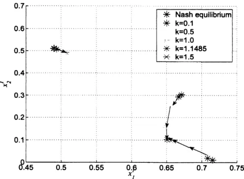
_{robust Nash equilibrium. Figure}

1 shows the trajectory ofplayer l’s strategies at _{the robust Nash equilibria for each} $k^{*3}$, in which

the verticalandhorizontal

axes

denote_{the first and second components of therobust Nash equilibria,}

respectively. Figure 1 indicates that two ofthe three equilibria

are

getting closer to each other

as

$k$

.

increases, and they almost coincide at $k=1.1485$

.

Furthermore, at $k=1.5$, the two equilibria

disappearandonlyone _{equilibrium is obtained.}

$*1$

Wecan_{find all Nash equilibria by usingabranchandbound basedapproach.} $*2$

Sinceweemployaniterativemethod,_wecanchoose anarbirrary startingpoint. Indeed,itisexpectedthatadifferent

startngpointcanleadtoadifferentsolution when theSOCCPhas multiple solutions.

$*3$

Table 1 Sizes ofuncertaintysetsand obtained robust Nash equilibria

Figure 1 Trajectory of player l’s strategiesatthe robust Nash equilibria

7 Concluding remarks

Inthis

paper, we

haveextendedtheconceptofrobustNash equilibrium to N-personnon-cooperative

gameswithnonlinearcostfunctions,andderivedsufficient conditionsforexistence and umiqueness of

the robust Nash equilibria by

means

of the GVIP

or

VIP reformulation techniques. In addition, we

have shown that the robust Nash equilibriumproblems with quadratic costfunctions and uncertainty

problem, and observedsomenumericalproperties.

We still have

some

fumre issues to be addressed. One importantissue is to weaken the sufficient

conditions foruniqueness oftherobustNash equilibrium. Infact, theuniquenessconditionsshown in

the

paper

are

rather restrictive, and there

seems

to remainmuch

room

for the improvement. Another

issue isto considerthe SOCCP reformulationforthe robust Nash equilibrium problemin whichboth

the cost function parameters and theopponents’ strategies

are

uncertain. In this

paper, we

have only

considered the

case

where either of them is uncertain. However, in the real situation, it would be

natural to

assume

thatboth of them involveuncertainties.

References

[1] M. AGHASSI AND D. BERTSIMAS, Robust game theory, Mathematical Programming, 107

(2006),

_pp.

_231-273.

[21 F. ALIZADEH AND D. GOLDFARB, Second-order

cone

programming, Mathematical

Program-ming,

95

(2003),

pp.

3-51.

[3] _J.-P. AUBIN,_{Mathematical Methods}

_of

_{Gameand EconomicTheory, North-Holland Publishing}

Company, Amsterdam, 1979.

[41 J.-P. AuBiN ANDH. FRANKOWSKA, Set-ValuedAnalysis, Birkhauser, 1990.

[5] A. BEN$-$TAL AND A. NEMiROvsKi,Robustsolutions

of

uncertainlinearprograms, Operations

ResearchLetters,25 (1999),

pp.

1-13.

[6] –, Selected topics in robust

convex

optimization, Mathematical Programming, 112 (2008),

pp. 125-158.

[7] D. P. BERTSEKAS, Convexanalysisandoptimization,AthenaScientific,_2003.

[8] L. ELGHAOUiAND H. LEBRET,Robustsolutionstoleast-squaresproblem withuncertaindata,

SIAMJoumal

on

Matrix AnalysisandApplications, 18 (1997),pp.

_1035-1064.

[9] F. FACCHINEI AND J.-S. PANG, Finite-Dimensional Variational Inequalities and

Complemen-tarityProblems,_{Springer-Verlag, New}York, 2003.

[10] _{S. C. FANG} AND E. L. PETERSON, _Generailizedvariational inequalities, Joumal of

optimiza-tion theory and applicaoptimiza-tions,38 (1982),pp.

363-383.

[11] M. FUKUSHIMA, Z.-Q. LUO, AND P. TSENG,Smoothing

_functionsfor

second-ordercone

com-plementarityproblems,SIAM Joumal

on

optimization, 12 (2001),

pp.

$436-i60$

.

[121 S. HAYASHI, N. YAMASHITA,ANDM. FuKusHiMA,A combinedsmoothing andregularization

methodfor

monotonesecond-orderconecomplementarityproblems,.SIAMJoumalon

Optimiza-tion, ₁₇₅ $(2\alpha)5)$,

pp.

335-353.

. [13] _–2 Robust Nash equilibria and second-order

cone

complementarlty problems, Joumal of

NonlinearandConvex Analysis, 6(2005),_{pp. 283-296.}

[14] _{R. NISHIMURA,S.} HAYAsHi, AND M. FUKUSHIMA,Robust Nash equilibria in N-person

non-cooperative games: Uniqueness and reformulation, Technical Report, 2008-003, Department

of AppliedMathematics andPhysics, Graduate School ofInformatics,KyotoUniversity, April,

2008.

[15] J. B. ROSEN, Existence and uniqueness

_of

equilibriumpoints

_for

concave

N-persons games,