Article
SimulationAnalysis Based on the EastAsian Macroeconometric Model China-Japan-US-Korea 4-Country Model
Taiyo OZAKI, Kyoto Gakuen University, Kyoto JAPAN [email protected]
Abstract :
The research is aimed at testing the properties of the Asian Link Model which has been developed since 2006, in which we deal with the model of Japan, the US, China and Korea and the bi-lateral trade linkage model. This model has expanded the conventional econometric model in several directions. One is to do farther investigation of changing bi-lateral trade patterns in more flexible form among those four countries. The second point is to use forward looking variables to evaluate the anticipated expectations to the new policy. The third is to add an energy model to simulate the future changes in theAsian economy with energy constraints.
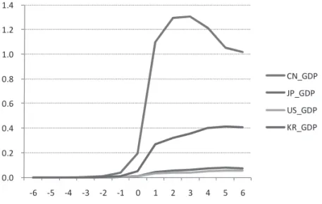
In this version, we mainly present the structures of the model and the simulation results of the stimulus packages which are just carried in the world. For example, the government investment by 1% of real GDP will lead the increase close to 1.3% in real GDP in the US economy, and so forth. As to the appreciation of RMB +10%, it will reduce the real GDP by 3
㹼5%. It is also notable that Chinese slowdown in exports leads the reduction in Korean exports simultaneously.
Keywords :
EastAsian Macroeconometric Model, forward-looking model, bi-lateral trade, stimulus package, simulation analysis
JEL : E17, F17, F18 Article
SimulationAnalysis Based on the EastAsian Macroeconometric Model China-Japan-US-Korea 4-Country Model
Taiyo OZAKI, Kyoto Gakuen University, Kyoto JAPAN [email protected]
Abstract :
The research is aimed at testing the properties of the Asian Link Model which has been developed since 2006, in which we deal with the model of Japan, the US, China and Korea and the bi-lateral trade linkage model. This model has expanded the conventional econometric model in several directions. One is to do farther investigation of changing bi-lateral trade patterns in more flexible form among those four countries. The second point is to use forward looking variables to evaluate the anticipated expectations to the new policy. The third is to add an energy model to simulate the future changes in theAsian economy with energy constraints.
In this version, we mainly present the structures of the model and the simulation results of the stimulus packages which are just carried in the world. For example, the government investment by 1% of real GDP will lead the increase close to 1.3% in real GDP in the US economy, and so forth. As to the appreciation of RMB +10%, it will reduce the real GDP by 3
㹼5%. It is also notable that Chinese slowdown in exports leads the reduction in Korean exports simultaneously.
Keywords :
EastAsian Macroeconometric Model, forward-looking model, bi-lateral trade, stimulus package, simulation analysis
JEL : E17, F17, F18 Article
Simulation Analysis Based on the East Asian Macroeconometric Model China-Japan-US-Korea 4-Country Model
Taiyo OZAKI, Kyoto Gakuen University, Kyoto JAPAN [email protected]
Abstract
The research is aimed at testing the properties of the Asian Link Model which has been developed since 2006, in which we deal with the model of Japan, the US, China and Korea and the bi-lateral trade linkage model.
This model has expanded the conventional econometric model in several directions. One is to do farther investigation of changing bi-lateral trade patterns in more flexible form among those four countries. The second point is to use forward looking variables to evaluate the anticipated expectations to the new policy. The third is to add an energy model to simulate the future changes in the Asian economy with energy constraints.
In this version, we mainly present the structures of the model and the simulation results of the stimulus packages which are just carried in the world. For example, the government investment by 1% of real GDP will lead the increase close to 1.3% in real GDP in the US economy, and so forth.
As to the appreciation of RMB +10%, it will reduce the real GDP by 3
㨪5%.
It is also notable that Chinese slowdown in exports leads the reduction in Korean exports simultaneously.
Keywords:
East Asian Macroeconometric Model, forward-looking model, bi-lateral trade, stimulus package, simulation analysis
JEL : E17, F17, F18
This research is supported by KAKENHI 20530223
1. Introduction
The research is aimed at testing the properties of the Asian Link Model which has been developed since 2005-2006, ( see Ozaki (2006)), in which we deal with the model of Japan, the US, China and Korea and the bi-lateral trade linkage model. The model is also designed for evaluating the recent fiscal stimulus packages.
This model has expanded conventional econometric models in several directions. One is to do farther investigation of changing bi-lateral trade patterns which include those four countries. The second point is that the model uses forward looking variables to evaluate the anticipated expectations to the new policy. The third is to add an energy model to simulate the future changes in the Asian economy with the excess energy use or the limited energy constraints.
The trade relation has been so dramatically changed that it is inevitable for many countries to assign the vertical structure of production system beyond nations and we must develop the new method which is more flexible and is able to evaluate properly the role of the third country effects.
2. Model and Specification (1) GDP definition
GDP=C+IF+GC+X -M
GDPV=CV+IFV+GCV+XV -MV
㺃㺃㺃
V denotes the nominal value. Do the same for the following.
CV=PC*C/100 IFV=PIF*IF/100 GCV=PGC*GC/100 XV=PX*X/100 MV=PM*M/100
(2) Consumption
Consumption function is formulated applying the Permanent Income Hypothesis, in which technically “model consistent” expectation ( sometimes confusing to Rational Expectation) is assumed. This type of the specification originally appeared in MULTIMOD, IMF (1998) , in which forward looking formulations are adopted.
The income constraint for a household is as follows;
1
(1 ) (1 )
t w t t t
W
t YL C r W
W ...wealth,
t
w...tax rate,
YL ...household income, C ...consumption,
r ...interest rate
We assumed to determine the consumption at the present time under the condition maximizing the discounted total utility/income in the future.
0
max 1 ( ) |
1
t
i C t i
i
E u C
E
d
¬ ¬
8
®
®
u ...utility function, E ...discount rate, 8 ...available information set
The expectation of the future gain is approximately substituted to the expectation of the series of the future income. There are many types of the expectation such as a typical distributed time-lag model, but, the most natural way to express the future income is to induce forward looking variables.
0 0
1 1
( ) | ) |
1 1
i i
t i t i t
i i
E u C E YL W
E E
d d
¬ ¬ ¬ ¬
8 8
® ®
® ®
¸ ¸
¹
·
¨ ¨
©
§ ¸
¹
¨ ·
©
§
¸
¹
¨ ·
©
§
¦f
0
) 1 1 (
1
1
i w t i ti
t
E t YL W
C G G
G
The final specification of the consumption function is given by
0 1 2
0
1 (1 )
1
i
t w t i t
i
C c c t YL c W
E
d
¬ ¬
® ® Brief notations using in EViews are as follows.
C=F( PEDYV/PC*100 Ȋ PENW(+i)/PC(+i)/(1+RLG(+i)) )
PEDY...disposable income, PENW....wealth, RLG.... interest rate Table 2.1 Consumption functions
Income t-value Wealth t-value
China 0.83 (*) with lag 0.005 0.48
Japan 0.88 (*) with lag 0.001 1.06
Korea 0.82 (*) without lag 0.049 2.06
US 1.04 (*) with lag 0.001 2.54
(*) propensity to consumption in the long run
PEDYV=PEWFP +PEOY -TY
PEWFP...wage income, PEOY...property income, TY...income tax SV=PEDYV-CV
PENW=PENW(-1)+SV SV....savings PEWFP=F( ER*ET )
ER....earnings per capita, ET....employee PEOY=F( RLB*PENW )
TY=F(PEDYV) (3) Investment
The ratio of the shadow value of capital to the unit of investment is known as the marginal Q, and this derives a linear relation between the marginal Q and the investment.
The marginal Q is defined by the following formulation originally developed in Behr and Bellgart (2002).
In the basic Q-model, the firm is assumed to maximize the expected value of the sum of discounted profits.
0
max 1 ) |
1
t
i t i i
Q
E Q
E
d
¬ ¬
8
®
®
Q ...corporate profit
We assume a Cobb-Douglas production function Y
tAK L
tB tC, and a profit function as follows,
t
p AK L
tB tCw L
t tq I
t tQ
p ...output price, K ...capital stock, L ...labor, w ...wage rate,
q ...unit cost of investment, I ...investment
The marginal productivity of capital, MPK, is given by
Y p Y Yp
p Y
K K Y K K
Q R
s s s s
s s s s
Here, we presume Yp x V (value added), then, the estimate of R is .
( )
e
i ii i
r d V K
R
The ratio of the shadow value of capital to the unit of investment is known as the marginal Q, and this derives a linear relation between the marginal Q and the investment.
The marginal Q is defined by the next formulation.
1 1
(1 ) e 1
( )
(1 ) (1 )
i
t i
t i i i
i t i t i
d V
Q E MPK
r R r K
d d
x
As d
td is assumed, the effect of the depreciation is absorbed in R e .Finally, we get the specification of the investment function.
0 1 2
1 1 1
1 (1 )
t i t
i i
t t i t
I GDP Z
K B B
dr K B K
¬
®
= + (1 - )
-1t t t t
K I d K
Z ...additional explanatory variables such as FDI and corporate operating surplus.
IF=IBUD +IFOR +ILON +IFF
IBUD...investment by the governmental fund IFOR...investment by the foreign capital ILON...investment by the private loan(?) IFF....private corporate investment
IFF/K(-1)=F( Ȋ GDP(i)/K(i)/(1+RLG(i)) Z(k)/K(-1) ) Ȋ GDP(i)/K(i)/(1+RLG(i))....proxy to marginal Q (Z(k))....additional elements such as...
Z1=COGTP Z2=RLB*PENW Z3=Money supply etc
Estimated parameters are as following.
( )
e
i ii i
r d V K
R
The ratio of the shadow value of capital to the unit of investment is known as the marginal Q, and this derives a linear relation between the marginal Q and the investment.
The marginal Q is defined by the next formulation.
1 1
(1 ) e 1
( )
(1 ) (1 )
i
t i
t i i i
i t i t i
d V
Q E MPK
r R r K
d d
x
As d
td is assumed, the effect of the depreciation is absorbed in R e .Finally, we get the specification of the investment function.
0 1 2
1 1 1
1 (1 )
t i t
i i
t t i t
I GDP Z
K B B
dr K B K
¬
®
= + (1 - )
-1t t t t
K I d K
Z ...additional explanatory variables such as FDI and corporate operating surplus.
IF=IBUD +IFOR +ILON +IFF
IBUD...investment by the governmental fund IFOR...investment by the foreign capital ILON...investment by the private loan(?) IFF....private corporate investment
IFF/K(-1)=F( Ȋ GDP(i)/K(i)/(1+RLG(i)) Z(k)/K(-1) ) Ȋ GDP(i)/K(i)/(1+RLG(i))....proxy to marginal Q (Z(k))....additional elements such as...
Z1=COGTP Z2=RLB*PENW Z3=Money supply etc
Estimated parameters are as following.
Table 2.2 Investment functions
Ȋ GDP(i)/K(i)/ t-value Z(k)/K(-1) t-value
China 0.53 11.4 13.9(**) 3.14
Japan 0.12 0.91 17.6(*) 1.50
Korea 0.11 1.15 48.9(**) 3.60
US 0.15 2.45 43.8(**) 2.83
(*) Z=Money supply (**) Z=corporate profit K=IFF+K(-1)
(China’s foreign investment) IFOR=F( GDP(i) W(i)/W(j) GDP(j) )
Foreign investment (FDI inflows) in China is substantially affected by Japan’s GDP.
Typical example is as follows;
log(IFOR)=-49.5-0.08*log(ER$/WWC$)+0.86*log(CN_GDP)+3.63*log(JP_GDP) In this estimation, CN_GDP is not significant, and its elasticity is rather low.
(4) Exports and Imports
Trade functions are formulated by each combination of trading partners. The row sum
of X
ch kr,, X
ch jp,is, for example, the total exports of China .Xij$ denotes the exports in
constant price of $ between i-j countries. The function contains indirect relative price combinations to reflect the substitution effect to the third party countries.
Figure 2.1 Trading partners, exports and imports
Consider a specific bi-lateral trade relation between (i) and (j) countries. Of course, the country (i) has several options regarding the trading partners importing/exporting goods.
㻯㼔㼕㼚㼍 㻶㼍㼜㼍㼚 㼁㻿 㻷㼛㼞㼑㼍 㻾㼃 㼃㼛㼞㼘㼐
㻯㼔㼕㼚㼍 㻙 㼀㻔㼏㻘㼖㻕
㻶㼍㼜㼍㼚 㼀㻔㼖㻘㼏㻕 㻙 㼀㻔㼖㻘㼡㻕 㼀㻔㼖㻘㼗㻕 㼀㻔㼖㻘㼞㻕 㼀㻔㼖㻘㼣㻕 㼄㼂㻐 㼀㼛㼠㼍㼘 㻱㼤㼜㼛㼞㼠
㼁㻿 㼀㻔㼡㻘㼖㻕 㻙
㻷㼛㼞㼑㼍 㼀㻔㼗㻘㼖㻕 㻙
㻾㼃 㼀㻔㼞㻘㼖㻕 㼀㼞㼞
㼃㼛㼞㼘㼐 㼀㻔㼣㻘㼖㻕
㻹 㼂㻐 㼀㼛㼍㼠㼍㼘 㻵㼙㼜㼛㼞㼠
In the conventional model, the formulation of export T
ij, or import T
jiis typically a
function of demand of the country(j) and the relative price
ij
p
p . This model implicitly implies that the domestic demand of j-country can be substituted by the foreign goods from i-country, but it does not tell how the change in i-j relation affects i-k relation explicitly.
To avoid this problem, we adopt the translog function formation to denote the j-i, i-k,...relations.
We assume a linear homogeneous function
1
,
2, M f M M "
M ...total real import, M
j...import from j-country, here, j=1,2,
To minimize the cost function of M , we use the translog function with 2nd order approximation, and this is denoted by
0 1 1 1
2 1
ln ln ln 1 ln
2
ln 1 ln ln ln
2
n n n
i i ij i j
i i j
n
M MM iM i
i
MV P PP
M M P M
B B H
B H H
MV ….total cost, namely total import in nominal term Using Shephard's lemma,
1
1
ln ln
ln ln
ln ln
i i i
i
i i
n
i ij i iM
j n
i ij i iM
j
P PM MV MV
P P MV MV S
P M
P GDP
B H H
B H H
s s s s
Here, we simply assume M f GDP ( ) . Parameter constraints are as follows, In the conventional model, the formulation of export T
ij, or import T
jiis typically a
function of demand of the country(j) and the relative price
ij
p
p . This model implicitly implies that the domestic demand of j-country can be substituted by the foreign goods from i-country, but it does not tell how the change in i-j relation affects i-k relation explicitly.
To avoid this problem, we adopt the translog function formation to denote the j-i, i-k,...relations.
We assume a linear homogeneous function
1
,
2, M f M M "
M ...total real import, M
j...import from j-country, here, j=1,2,
To minimize the cost function of M , we use the translog function with 2nd order approximation, and this is denoted by
0 1 1 1
2 1
ln ln ln 1 ln
2
ln 1 ln ln ln
2
n n n
i i ij i j
i i j
n
M MM iM i
i
MV P PP
M M P M
B B H
B H H
MV ….total cost, namely total import in nominal term Using Shephard's lemma,
1
1
ln ln
ln ln
ln ln
i i i
i
i i
n
i ij i iM
j n
i ij i iM
j
P PM
MV MV S
P P MV MV
P M
P GDP
B H H
B H H
s s s s
Here, we simply assume M f GDP ( ) . Parameter constraints are as follows,
In the conventional model, the formulation of export T
ij, or import T
jiis typically a
function of demand of the country(j) and the relative price
ij
p
p . This model implicitly implies that the domestic demand of j-country can be substituted by the foreign goods from i-country, but it does not tell how the change in i-j relation affects i-k relation explicitly.
To avoid this problem, we adopt the translog function formation to denote the j-i, i-k,...relations.
We assume a linear homogeneous function
1
,
2, M f M M "
M ...total real import, M
j...import from j-country, here, j=1,2,
To minimize the cost function of M , we use the translog function with 2nd order approximation, and this is denoted by
0 1 1 1
2 1
ln ln ln 1 ln
2
ln 1 ln ln ln
2
n n n
i i ij i j
i i j
n
M MM iM i
i
MV P PP
M M P M
B B H
B H H
MV ….total cost, namely total import in nominal term Using Shephard's lemma,
1
1
ln ln
ln ln
ln ln
i i i
i
i i
n
i ij i iM
j n
i ij i iM
j
P PM
MV MV S
P P MV MV
P M
P GDP
B H H
B H H
s s s s
Here, we simply assume M f GDP ( ) .
Parameter constraints are as follows,
Table 2.2 Investment functions
Ȋ GDP(i)/K(i)/ t-value Z(k)/K(-1) t-value
China 0.53 11.4 13.9(**) 3.14
Japan 0.12 0.91 17.6(*) 1.50
Korea 0.11 1.15 48.9(**) 3.60
US 0.15 2.45 43.8(**) 2.83
(*) Z=Money supply (**) Z=corporate profit K=IFF+K(-1)
(China’s foreign investment) IFOR=F( GDP(i) W(i)/W(j) GDP(j) )
Foreign investment (FDI inflows) in China is substantially affected by Japan’s GDP.
Typical example is as follows;
log(IFOR)=-49.5-0.08*log(ER$/WWC$)+0.86*log(CN_GDP)+3.63*log(JP_GDP) In this estimation, CN_GDP is not significant, and its elasticity is rather low.
(4) Exports and Imports
Trade functions are formulated by each combination of trading partners. The row sum
of X
ch kr,, X
ch jp,is, for example, the total exports of China .Xij$ denotes the exports in
constant price of $ between i-j countries. The function contains indirect relative price combinations to reflect the substitution effect to the third party countries.
Figure 2.1 Trading partners, exports and imports
Consider a specific bi-lateral trade relation between (i) and (j) countries. Of course, the country (i) has several options regarding the trading partners importing/exporting goods.
㻯㼔㼕㼚㼍 㻶㼍㼜㼍㼚 㼁㻿 㻷㼛㼞㼑㼍 㻾㼃 㼃㼛㼞㼘㼐
㻯㼔㼕㼚㼍 㻙 㼀㻔㼏㻘㼖㻕
㻶㼍㼜㼍㼚 㼀㻔㼖㻘㼏㻕 㻙 㼀㻔㼖㻘㼡㻕 㼀㻔㼖㻘㼗㻕 㼀㻔㼖㻘㼞㻕 㼀㻔㼖㻘㼣㻕 㼄㼂㻐 㼀㼛㼠㼍㼘 㻱㼤㼜㼛㼞㼠
㼁㻿 㼀㻔㼡㻘㼖㻕 㻙
㻷㼛㼞㼑㼍 㼀㻔㼗㻘㼖㻕 㻙
㻾㼃 㼀㻔㼞㻘㼖㻕 㼀㼞㼞
㼃㼛㼞㼘㼐 㼀㻔㼣㻘㼖㻕
㻹 㼂㻐 㼀㼛㼍㼠㼍㼘 㻵㼙㼜㼛㼞㼠
In the conventional model, the formulation of export T
ij, or import T
jiis typically a
function of demand of the country(j) and the relative price
ij
p
p . This model implicitly implies that the domestic demand of j-country can be substituted by the foreign goods from i-country, but it does not tell how the change in i-j relation affects i-k relation explicitly.
To avoid this problem, we adopt the translog function formation to denote the j-i, i-k,...relations.
We assume a linear homogeneous function
1
,
2, M f M M "
M ...total real import, M
j...import from j-country, here, j=1,2,
To minimize the cost function of M , we use the translog function with 2nd order approximation, and this is denoted by
0 1 1 1
2 1
ln ln ln 1 ln
2
ln 1 ln ln ln
2
n n n
i i ij i j
i i j
n
M MM iM i
i
MV P PP
M M P M
B B H
B H H
MV ….total cost, namely total import in nominal term Using Shephard's lemma,
1
1
ln ln
ln ln
ln ln
i i i
i
i i
n
i ij i iM
j n
i ij i iM
j
P PM MV MV
P P MV MV S
P M
P GDP
B H H
B H H
s s s s
Here, we simply assume M f GDP ( ) .
Parameter constraints are as follows,
1
1
1
1 0
0
n i i
n j ij
n i iM
B H H
The sum of j column of T(i,j) is the total imports of j country. Each element reflects the exporting price of respective country, which differs from each other and forms the composite import price.
Crude oil and natural gas are imported from the rest of the world and separately treated to evaluate the effect of oil price changes.
(Example of China)
CN_M$V=T(jpcn)$+T(krch)$+T(usch)$+T(rsch)$
CN_M$=T(jpch)$/JP_PX$*100+T(krch)$/KR_PX$*100+T(usch)$/US_PX$(us)*100 +XVrsch$
MVrsch$=MOIL$+MGAS$+MCOAL$ + Mrsch_others$
CN_PM$=CN_MV$/CN_M$*100 PM=F( CN_PM$*CN_RXD) MV=F(CN_M$V*CN_RXD) M=MV/PM*100
(5) Recent changes in the trading pattern
Drastic changes in the trading patterns have taken place since 1995. Table 2.3 shows that the role of China is becoming greater rapidly in exports/imports to/from the US and World.Accompanied by this, Korea has enforced its dependency to China.
Japan especially raises exports in the area of industrial supplies (BEC classification), this causes the increase in imports of equipments and parts through FDI.
Regarding consumption goods, relation between China and the US and Korea has enhanced compared to the relation between China and Jpanan.
Table 2.3 Changes in the trading pattern
㻞㻜㻜㻡㻛㻝㻥㻥㻡 㻮㻱㻯㻝 㻲㼛㼛㼐 㼍㼚㼐 㻮㼑㼢㼑㼞㼍㼓㼑㻯㻺 㻶㻼 㻷㻾 㼁㻿 㼃㼛㼞㼘㼐
㻯㻺 㻝㻚㻣㻠 㻠㻚㻣㻟 㻠㻚㻡㻝 㻞㻚㻜㻢
㻶㻼 㻠㻚㻟㻥 㻟㻚㻠㻠 㻝㻚㻢㻡 㻝㻚㻡㻢
㻷㻾 㻞㻚㻥㻥 㻜㻚㻣㻟 㻝㻚㻣㻣 㻜㻚㻥㻤
㼁㻿 㻟㻚㻜㻣 㻜㻚㻢㻣 㻝㻚㻜㻥 㻝㻚㻞㻟
㼃㼛㼞㼘㼐 㻞㻚㻢㻟 㻜㻚㻥㻣 㻝㻚㻤㻞 㻝㻚㻥㻥 㻝㻚㻠㻣
㻞㻜㻜㻡㻛㻝㻥㻥㻡 㻮㻱㻯㻞 㻵㼚㼐㼡㼟㼠㼞㼕㼍㼘 㻿㼡㼜㼜㼘㼕㼑㼟
㻯㻺 㻶㻼 㻷㻾 㼁㻿 㼃㼛㼞㼘㼐
㻯㻺 㻞㻚㻢㻠 㻟㻚㻢㻞 㻢㻚㻢㻣 㻟㻚㻥㻜
㻶㻼 㻟㻚㻟㻥 㻝㻚㻥㻥 㻝㻚㻝㻣 㻝㻚㻡㻡
㻷㻾 㻟㻚㻣㻡 㻝㻚㻠㻠 㻞㻚㻠㻥 㻝㻚㻤㻝
㼁㻿 㻟㻚㻞㻝 㻜㻚㻤㻠 㻜㻚㻥㻡 㻝㻚㻡㻡
㼃㼛㼞㼘㼐 㻟㻚㻤㻤 㻝㻚㻝㻥 㻝㻚㻡㻥 㻞㻚㻝㻡 㻝㻚㻡㻡
㻞㻜㻜㻡㻛㻝㻥㻥㻡 㻮㻱㻯㻟 㻲㼡㼑㼘㼟
㻯㻺 㻶㻼 㻷㻾 㼁㻿 㼃㼛㼞㼘㼐
㻯㻺 㻝㻚㻡㻣 㻟㻚㻞㻟 㻞㻚㻞㻥 㻟㻚㻞㻢
㻶㻼 㻠㻚㻜㻞 㻜㻚㻡㻤 㻞㻚㻤㻥 㻝㻚㻣㻞
㻷㻾 㻢㻚㻢㻠 㻠㻚㻝㻜 㻝㻤㻚㻥㻢 㻢㻚㻠㻢
㼁㻿 㻣㻚㻜㻢 㻜㻚㻡㻤 㻜㻚㻢㻢 㻞㻚㻣㻝
㼃㼛㼞㼘㼐 㻝㻞㻚㻡㻡 㻞㻚㻠㻣 㻟㻚㻡㻝 㻠㻚㻣㻟 㻠㻚㻜㻤
㻞㻜㻜㻡㻛㻝㻥㻥㻡 㻮㻱㻯㻠 㻯㼍㼜㼕㼠㼍㼘 㼓㼛㼛㼐㼟 㼍㼚㼐 㻼㼍㼞㼠㼟
㻯㻺 㻶㻼 㻷㻾 㼁㻿 㼃㼛㼞㼘㼐
㻯㻺 㻣㻚㻟㻣 㻞㻜㻚㻤㻤 㻝㻟㻚㻠㻟 㻝㻞㻚㻞㻞
㻶㻼 㻟㻚㻣㻝 㻝㻚㻝㻣 㻜㻚㻣㻤 㻝㻚㻝㻝
㻷㻾 㻝㻤㻚㻜㻥 㻝㻚㻤㻢 㻝㻚㻝㻥 㻞㻚㻢㻥
㼁㻿 㻟㻚㻣㻥 㻜㻚㻤㻤 㻝㻚㻞㻡 㻝㻚㻠㻡
㼃㼛㼞㼘㼐 㻢㻚㻞㻡 㻝㻚㻤㻡 㻝㻚㻣㻣 㻝㻚㻣㻡 㻝㻚㻡㻤
㻞㻜㻜㻡㻛㻝㻥㻥㻡 㻮㻱㻯㻡 㼀㼞㼍㼚㼟㼜㼛㼞㼠 㼑㼝㼡㼕㼜㼙㼑㼚㼠 㼍㼚㼐 㻼㼍㼞㼠㼟
㻯㻺 㻶㻼 㻷㻾 㼁㻿 㼃㼛㼞㼘㼐
㻯㻺 㻥㻚㻞㻞 㻝㻜㻚㻡㻥 㻤㻚㻢㻢 㻤㻚㻟㻞
㻶㻼 㻠㻚㻜㻣 㻝㻚㻡㻞 㻝㻚㻠㻢 㻝㻚㻠㻣
㻷㻾 㻝㻟㻚㻢㻤 㻞㻚㻝㻢 㻟㻚㻢㻠 㻟㻚㻝㻜
㼁㻿 㻠㻚㻝㻜 㻝㻚㻜㻝 㻜㻚㻥㻣 㻝㻚㻣㻥
㼃㼛㼞㼘㼐 㻠㻚㻥㻥 㻝㻚㻠㻣 㻝㻚㻝㻠 㻝㻚㻥㻢 㻞㻚㻜㻝
㻞㻜㻜㻡㻛㻝㻥㻥㻡 㻮㻱㻯㻢 㻯㼛㼚㼟㼡㼙㼜㼠㼕㼛㼚 㼓㼛㼛㼐㼟
㻯㻺 㻶㻼 㻷㻾 㼁㻿 㼃㼛㼞㼘㼐
㻯㻺 㻞㻚㻞㻜 㻠㻚㻟㻡 㻠㻚㻠㻞 㻟㻚㻢㻠
㻶㻼 㻝㻚㻡㻥 㻝㻚㻤㻟 㻝㻚㻡㻠 㻝㻚㻠㻡
㻷㻾 㻞㻚㻥㻢 㻜㻚㻠㻢 㻜㻚㻤㻥 㻜㻚㻥㻢
㼁㻿 㻡㻚㻠㻡 㻜㻚㻤㻟 㻝㻚㻜㻥 㻝㻚㻡㻣
㼃㼛㼞㼘㼐 㻟㻚㻟㻢 㻝㻚㻟㻤 㻞㻚㻠㻜 㻞㻚㻟㻣 㻞㻚㻝㻜
㻞㻜㻜㻡㻛㻝㻥㻥㻡 㻮㻱㻯 㼀㼛㼠㼍㼘
㻯㻺 㻶㻼 㻷㻾 㼁㻿 㼃㼛㼞㼘㼐
㻯㻺 㻞㻚㻥㻡 㻡㻚㻞㻡 㻢㻚㻢㻜 㻡㻚㻝㻞
㻶㻼 㻟㻚㻢㻠 㻝㻚㻠㻥 㻝㻚㻝㻝 㻝㻚㻟㻠
㻷㻾 㻢㻚㻣㻣 㻝㻚㻠㻝 㻝㻚㻣㻜 㻞㻚㻞㻣
㼁㻿 㻟㻚㻡㻢 㻜㻚㻤㻢 㻝㻚㻜㻥 㻝㻚㻡㻡
㼃㼛㼞㼘㼐 㻡㻚㻜㻜 㻝㻚㻡㻟 㻝㻚㻥㻟 㻞㻚㻞㻡 㻝㻚㻤㻝
1
1
1
1 0
0
n i i
n j ij
n i iM
B H H
The sum of j column of T(i,j) is the total imports of j country. Each element reflects the exporting price of respective country, which differs from each other and forms the composite import price.
Crude oil and natural gas are imported from the rest of the world and separately treated to evaluate the effect of oil price changes.
(Example of China)
CN_M$V=T(jpcn)$+T(krch)$+T(usch)$+T(rsch)$
CN_M$=T(jpch)$/JP_PX$*100+T(krch)$/KR_PX$*100+T(usch)$/US_PX$(us)*100 +XVrsch$
MVrsch$=MOIL$+MGAS$+MCOAL$ + Mrsch_others$
CN_PM$=CN_MV$/CN_M$*100 PM=F( CN_PM$*CN_RXD) MV=F(CN_M$V*CN_RXD) M=MV/PM*100
(5) Recent changes in the trading pattern
Drastic changes in the trading patterns have taken place since 1995. Table 2.3 shows that the role of China is becoming greater rapidly in exports/imports to/from the US and World.Accompanied by this, Korea has enforced its dependency to China.
Japan especially raises exports in the area of industrial supplies (BEC classification), this causes the increase in imports of equipments and parts through FDI.
Regarding consumption goods, relation between China and the US and Korea has enhanced compared to the relation between China and Jpanan.
Table 2.3 Changes in the trading pattern
㻞㻜㻜㻡㻛㻝㻥㻥㻡 㻮㻱㻯㻝 㻲㼛㼛㼐 㼍㼚㼐 㻮㼑㼢㼑㼞㼍㼓㼑㻯㻺 㻶㻼 㻷㻾 㼁㻿 㼃㼛㼞㼘㼐
㻯㻺 㻝㻚㻣㻠 㻠㻚㻣㻟 㻠㻚㻡㻝 㻞㻚㻜㻢
㻶㻼 㻠㻚㻟㻥 㻟㻚㻠㻠 㻝㻚㻢㻡 㻝㻚㻡㻢
㻷㻾 㻞㻚㻥㻥 㻜㻚㻣㻟 㻝㻚㻣㻣 㻜㻚㻥㻤
㼁㻿 㻟㻚㻜㻣 㻜㻚㻢㻣 㻝㻚㻜㻥 㻝㻚㻞㻟
㼃㼛㼞㼘㼐 㻞㻚㻢㻟 㻜㻚㻥㻣 㻝㻚㻤㻞 㻝㻚㻥㻥 㻝㻚㻠㻣
㻞㻜㻜㻡㻛㻝㻥㻥㻡 㻮㻱㻯㻞 㻵㼚㼐㼡㼟㼠㼞㼕㼍㼘 㻿㼡㼜㼜㼘㼕㼑㼟
㻯㻺 㻶㻼 㻷㻾 㼁㻿 㼃㼛㼞㼘㼐
㻯㻺 㻞㻚㻢㻠 㻟㻚㻢㻞 㻢㻚㻢㻣 㻟㻚㻥㻜
㻶㻼 㻟㻚㻟㻥 㻝㻚㻥㻥 㻝㻚㻝㻣 㻝㻚㻡㻡
㻷㻾 㻟㻚㻣㻡 㻝㻚㻠㻠 㻞㻚㻠㻥 㻝㻚㻤㻝
㼁㻿 㻟㻚㻞㻝 㻜㻚㻤㻠 㻜㻚㻥㻡 㻝㻚㻡㻡
㼃㼛㼞㼘㼐 㻟㻚㻤㻤 㻝㻚㻝㻥 㻝㻚㻡㻥 㻞㻚㻝㻡 㻝㻚㻡㻡
㻞㻜㻜㻡㻛㻝㻥㻥㻡 㻮㻱㻯㻟 㻲㼡㼑㼘㼟
㻯㻺 㻶㻼 㻷㻾 㼁㻿 㼃㼛㼞㼘㼐
㻯㻺 㻝㻚㻡㻣 㻟㻚㻞㻟 㻞㻚㻞㻥 㻟㻚㻞㻢
㻶㻼 㻠㻚㻜㻞 㻜㻚㻡㻤 㻞㻚㻤㻥 㻝㻚㻣㻞
㻷㻾 㻢㻚㻢㻠 㻠㻚㻝㻜 㻝㻤㻚㻥㻢 㻢㻚㻠㻢
㼁㻿 㻣㻚㻜㻢 㻜㻚㻡㻤 㻜㻚㻢㻢 㻞㻚㻣㻝
㼃㼛㼞㼘㼐 㻝㻞㻚㻡㻡 㻞㻚㻠㻣 㻟㻚㻡㻝 㻠㻚㻣㻟 㻠㻚㻜㻤
㻞㻜㻜㻡㻛㻝㻥㻥㻡 㻮㻱㻯㻠 㻯㼍㼜㼕㼠㼍㼘 㼓㼛㼛㼐㼟 㼍㼚㼐 㻼㼍㼞㼠㼟
㻯㻺 㻶㻼 㻷㻾 㼁㻿 㼃㼛㼞㼘㼐
㻯㻺 㻣㻚㻟㻣 㻞㻜㻚㻤㻤 㻝㻟㻚㻠㻟 㻝㻞㻚㻞㻞
㻶㻼 㻟㻚㻣㻝 㻝㻚㻝㻣 㻜㻚㻣㻤 㻝㻚㻝㻝
㻷㻾 㻝㻤㻚㻜㻥 㻝㻚㻤㻢 㻝㻚㻝㻥 㻞㻚㻢㻥
㼁㻿 㻟㻚㻣㻥 㻜㻚㻤㻤 㻝㻚㻞㻡 㻝㻚㻠㻡
㼃㼛㼞㼘㼐 㻢㻚㻞㻡 㻝㻚㻤㻡 㻝㻚㻣㻣 㻝㻚㻣㻡 㻝㻚㻡㻤
㻞㻜㻜㻡㻛㻝㻥㻥㻡 㻮㻱㻯㻡 㼀㼞㼍㼚㼟㼜㼛㼞㼠 㼑㼝㼡㼕㼜㼙㼑㼚㼠 㼍㼚㼐 㻼㼍㼞㼠㼟
㻯㻺 㻶㻼 㻷㻾 㼁㻿 㼃㼛㼞㼘㼐
㻯㻺 㻥㻚㻞㻞 㻝㻜㻚㻡㻥 㻤㻚㻢㻢 㻤㻚㻟㻞
㻶㻼 㻠㻚㻜㻣 㻝㻚㻡㻞 㻝㻚㻠㻢 㻝㻚㻠㻣
㻷㻾 㻝㻟㻚㻢㻤 㻞㻚㻝㻢 㻟㻚㻢㻠 㻟㻚㻝㻜
㼁㻿 㻠㻚㻝㻜 㻝㻚㻜㻝 㻜㻚㻥㻣 㻝㻚㻣㻥
㼃㼛㼞㼘㼐 㻠㻚㻥㻥 㻝㻚㻠㻣 㻝㻚㻝㻠 㻝㻚㻥㻢 㻞㻚㻜㻝
㻞㻜㻜㻡㻛㻝㻥㻥㻡 㻮㻱㻯㻢 㻯㼛㼚㼟㼡㼙㼜㼠㼕㼛㼚 㼓㼛㼛㼐㼟
㻯㻺 㻶㻼 㻷㻾 㼁㻿 㼃㼛㼞㼘㼐
㻯㻺 㻞㻚㻞㻜 㻠㻚㻟㻡 㻠㻚㻠㻞 㻟㻚㻢㻠
㻶㻼 㻝㻚㻡㻥 㻝㻚㻤㻟 㻝㻚㻡㻠 㻝㻚㻠㻡
㻷㻾 㻞㻚㻥㻢 㻜㻚㻠㻢 㻜㻚㻤㻥 㻜㻚㻥㻢
㼁㻿 㻡㻚㻠㻡 㻜㻚㻤㻟 㻝㻚㻜㻥 㻝㻚㻡㻣
㼃㼛㼞㼘㼐 㻟㻚㻟㻢 㻝㻚㻟㻤 㻞㻚㻠㻜 㻞㻚㻟㻣 㻞㻚㻝㻜
㻞㻜㻜㻡㻛㻝㻥㻥㻡 㻮㻱㻯 㼀㼛㼠㼍㼘
㻯㻺 㻶㻼 㻷㻾 㼁㻿 㼃㼛㼞㼘㼐
㻯㻺 㻞㻚㻥㻡 㻡㻚㻞㻡 㻢㻚㻢㻜 㻡㻚㻝㻞
㻶㻼 㻟㻚㻢㻠 㻝㻚㻠㻥 㻝㻚㻝㻝 㻝㻚㻟㻠
㻷㻾 㻢㻚㻣㻣 㻝㻚㻠㻝 㻝㻚㻣㻜 㻞㻚㻞㻣
㼁㻿 㻟㻚㻡㻢 㻜㻚㻤㻢 㻝㻚㻜㻥 㻝㻚㻡㻡
㼃㼛㼞㼘㼐 㻡㻚㻜㻜 㻝㻚㻡㻟 㻝㻚㻥㻟 㻞㻚㻞㻡 㻝㻚㻤㻝
(6) Tax and Financial sector (Example of China)
TAXES=TXAV+TXIV+TXTV+TY+TXOTH+TINT TXAV...tax on the agricultural sctor
TXIV...tax on industry and commerce TXTV...tariff on trade
TY...income tax
TXOTH...tax, miscellaneous TINT...tax on interest GREV=TAXES+GREVO GEXP=GCV+GIV+GEOTH GB=GBPRIM
=GREV-GEXP =-(GGDBTX) =GGDBT-GGDBT(-1) (7) Money demand and interest rate
We chose the model with the monetary policy rule formulated originally by Clarida, Galf and Geltler (2000) and re-quoted in Cho and Moreno (2006). Theoretical model is as following,
1
(1 )[
1]
t t t t MP
R B S R
S C E p
C ygap F
R
tis the combination of the past interest rate and the expected inflation rate and the deviation of output from trend or the potential output. F
MPis the monetary policy rules or the monetary shocks. The parameter Ș denotes the long run reaction of the central bank to the expected inflation, and also, ș denotes the measure to evaluate the effects of the deviation of the output from the potential output, here we adopt the money supply as a proxy instead of GDP gap.
(Short term interest rate)
RSH=F( Ș RSH(-1) (1- Ș )PGDP(+1)/PGDP ș MON/PGDP)
Table 2.4 Interest function
Ș t-value ș t-value
China 0.63 3.28 -0.99 -1.66
Japan 0.68 6.43 -1.50 -1.59
Korea 0.59 9.70 -3.51 -7.11
US 0.59 6.01 -2.16 -1.00
(Long term interest rate)
RLG=F( Ș RLG(+1) (1-Ș )RLG(-1) șRSH )
(8) Balance of payment
RES$=RES$(-1)+BCU$+BCAP$
BCU$=X$V-M$V
X$V...nominal export in dollar M$V...nominal import in dollar BCAP$=FDI$+NFDI$
(9) Deflator and price index
The equation for the price deflator is an application of the expanded Phillips theory.
1
(1 )
1t t t t t
p E E p
E p
M ygap F
This type of formulation is proposed in Calvo(1983) and Cho and Moreno (2006) in the context of the aggregate supply equation of new Keynesian macro models. Here, we propose tentatively that the deflator PIF can be formulated like those.
PGDP=GDPV/GDP*100 PX....exogenous
PM....determined by the trade sector, a combination of the price of exporting countries.
PC=F( PC(-1) ER ) ER...earning, wage PIF=F( PM ER) PGC=F( PC )
(10) Earnings
ER=F( GDPV/ET GDPGAP ) GDPHAT= Ȋ GDP(j)/3
World average wage index (exogenous here)
WW$=F( ER(ch)/RXD(ch) ER(jp)/RXD(jp) ER(kr)/RXD(kr) ER(us)/RXD(us) ) WW$(ch)=F( ER(ch)/RXD(ch) )
(11) Labor
ET=F( GDP GDP(-1)/ET(-1) ) U=LS-ET
URATE=U/LS*100
(6) Tax and Financial sector (Example of China)
TAXES=TXAV+TXIV+TXTV+TY+TXOTH+TINT TXAV...tax on the agricultural sctor
TXIV...tax on industry and commerce TXTV...tariff on trade
TY...income tax
TXOTH...tax, miscellaneous TINT...tax on interest GREV=TAXES+GREVO GEXP=GCV+GIV+GEOTH GB=GBPRIM
=GREV-GEXP =-(GGDBTX) =GGDBT-GGDBT(-1) (7) Money demand and interest rate
We chose the model with the monetary policy rule formulated originally by Clarida, Galf and Geltler (2000) and re-quoted in Cho and Moreno (2006). Theoretical model is as following,
1
(1 )[
1]
t t t t MP
R B S R
S C E p
C ygap F
R
tis the combination of the past interest rate and the expected inflation rate and the deviation of output from trend or the potential output. F
MPis the monetary policy rules or the monetary shocks. The parameter Ș denotes the long run reaction of the central bank to the expected inflation, and also, ș denotes the measure to evaluate the effects of the deviation of the output from the potential output, here we adopt the money supply as a proxy instead of GDP gap.
(Short term interest rate)
RSH=F( Ș RSH(-1) (1- Ș )PGDP(+1)/PGDP ș MON/PGDP)
Table 2.4 Interest function
Ș t-value ș t-value
China 0.63 3.28 -0.99 -1.66
Japan 0.68 6.43 -1.50 -1.59
Korea 0.59 9.70 -3.51 -7.11
US 0.59 6.01 -2.16 -1.00
(Long term interest rate)
RLG=F( Ș RLG(+1) (1-Ș)RLG(-1) ș RSH )
(8) Balance of payment
RES$=RES$(-1)+BCU$+BCAP$
BCU$=X$V-M$V
X$V...nominal export in dollar M$V...nominal import in dollar BCAP$=FDI$+NFDI$
(9) Deflator and price index
The equation for the price deflator is an application of the expanded Phillips theory.
1
(1 )
1t t t t t
p E E p
E p
M ygap F
This type of formulation is proposed in Calvo(1983) and Cho and Moreno (2006) in the context of the aggregate supply equation of new Keynesian macro models. Here, we propose tentatively that the deflator PIF can be formulated like those.
PGDP=GDPV/GDP*100 PX....exogenous
PM....determined by the trade sector, a combination of the price of exporting countries.
PC=F( PC(-1) ER ) ER...earning, wage PIF=F( PM ER) PGC=F( PC )
(10) Earnings
ER=F( GDPV/ET GDPGAP ) GDPHAT= Ȋ GDP(j)/3
World average wage index (exogenous here)
WW$=F( ER(ch)/RXD(ch) ER(jp)/RXD(jp) ER(kr)/RXD(kr) ER(us)/RXD(us) ) WW$(ch)=F( ER(ch)/RXD(ch) )
(11) Labor
ET=F( GDP GDP(-1)/ET(-1) ) U=LS-ET
URATE=U/LS*100
ET....employee U....unemployment LS....labor supply
(12) Energy demand
Both of the translog approach and the conventional specification are tested to denote the substitutable relation between energy sources.
TDMD$=DOIL*POIL$+DCCAL*PCOAL$+DGAS*PGAS$
DOIL, DGAS, DCOAL....demand for crude oil, gas, coal in mtoe DOIL*POIL$/TDMD$=F( GDP PGDP$ Ȋ P$(j) )
DCOAL*PCOAL$/TDMD$=F( GDP PGDP$ Ȋ P$(j) ) DGAS*PGAS$/TDMD$=F( GDP PGDP$ Ȋ P$(j) )
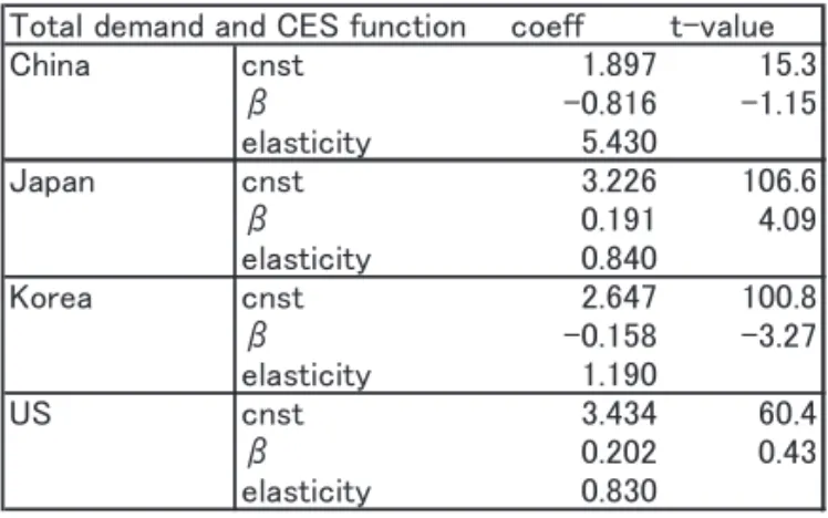
We also tried to estimate the parameter ș directly using CES function.
\ ^
10 coal gas oil
TPEN A w DCOAL
Cw DGAS
Cw DOIL
C C1 / (1 )
F C
TPEN Total energy demand (mtoe)
DOIL primary energy demand for Oil (mtoe) DGAS primary energy demand for Gas (mtoe) DCOAL primary energy demand for Coal (mtoe)
Table 2.5 Elasticity of substitution
Elasticity of substitution can vary depending on the nation's stage of development. China still seems to have high possibility of substitution among energy sources.
㼀㼛㼠㼍㼘 㼐㼑㼙㼍㼚㼐 㼍㼚㼐 㻯㻱㻿 㼒㼡㼚㼏㼠㼕㼛㼚 㼏㼛㼑㼒㼒 㼠㻙㼢㼍㼘㼡㼑
㻯㼔㼕㼚㼍 㼏㼚㼟㼠 㻝㻚㻤㻥㻣 㻝㻡㻚㻟
䃑 㻙㻜㻚㻤㻝㻢 㻙㻝㻚㻝㻡
㼑㼘㼍㼟㼠㼕㼏㼕㼠㼥 㻡㻚㻠㻟㻜
㻶㼍㼜㼍㼚 㼏㼚㼟㼠 㻟㻚㻞㻞㻢 㻝㻜㻢㻚㻢
䃑 㻜㻚㻝㻥㻝 㻠㻚㻜㻥
㼑㼘㼍㼟㼠㼕㼏㼕㼠㼥 㻜㻚㻤㻠㻜
㻷㼛㼞㼑㼍 㼏㼚㼟㼠 㻞㻚㻢㻠㻣 㻝㻜㻜㻚㻤
䃑 㻙㻜㻚㻝㻡㻤 㻙㻟㻚㻞㻣
㼑㼘㼍㼟㼠㼕㼏㼕㼠㼥 㻝㻚㻝㻥㻜
㼁㻿 㼏㼚㼟㼠 㻟㻚㻠㻟㻠 㻢㻜㻚㻠
䃑 㻜㻚㻞㻜㻞 㻜㻚㻠㻟
㼑㼘㼍㼟㼠㼕㼏㼕㼠㼥 㻜㻚㻤㻟㻜
3. Testing the Model
To test and simulate the model, we need a little complicated procedure to deal with forward looking variables, which is originally developed in Fair (1984) and sometimes called “extended path method”. This method calculates the future expected values to determine the present value of endogenous variables, therefore, for example, future GDP affects present consumption because we usually anticipate policy changes in the future.
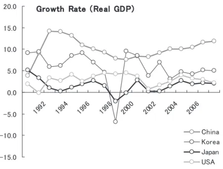
We carried the final test from 1990 to 2006, results of GDPs as a base line of each country are presented in the following page.
In the Asian model it seems rather difficult to pursuit the deep trough during the crisis 1997-1999.
Figure 3.1 Growth rate of 4 countries
MAPE (Mean Absolute Percent Error) regarding principal endogenous variables are shown in the table.
Table 3.1 MAPE
(*) MAPE stands for the mean absolute percent errors (%) 㻳㼞㼛㼣㼠㼔 㻾㼍㼠㼑 㻔 㻾㼑㼍㼘 㻳㻰㻼㻕
㻙㻝㻡㻚㻜 㻙㻝㻜㻚㻜 㻙㻡㻚㻜 㻜㻚㻜 㻡㻚㻜 㻝㻜㻚㻜 㻝㻡㻚㻜 㻞㻜㻚㻜
㻝㻥㻥㻞 㻝㻥㻥㻠
㻝㻥㻥㻢 㻝㻥㻥㻤
㻞㻜㻜㻜 㻞㻜㻜㻞
㻞㻜㻜㻠 㻞㻜㻜㻢
㻯㼔㼕㼚㼍 㻷㼛㼞㼑㼍 㻶㼍㼜㼍㼚 㼁㻿㻭


![¯]^°uv amp;#'&](data:image/gif;base64,R0lGODlhAQABAIAAAP///wAAACH5BAEAAAAALAAAAAABAAEAAAICRAEAOw==)