Finestructure Variability

Oceanography

T H E I N D O N E S I A N S E A S

Indonesian Seas

Finestructure Variability

The Indonesian seas contain evidence of enhanced vertical mixing. Coupled with the highly stratifi ed tropical thermocline, this enhanced mixing implies large verti- cal fl uxes of heat and buoyancy from the ocean-atmosphere boundary downward

B Y A M Y F F I E L D A N D R O B I N R O B E R T S O N

deep into the water column. To accu- rately predict climate change requires quantifying this vertical mixing and its temporal and spatial variability, because these fl uxes help regulate ocean heat storage and thermohaline circulation.

We use 18 years of temperature stratifi - cation data from expendable bathyther- mographic (XBT) probes to show that the fi nestructure associated with mixing reveals clear enhancement near topogra- phy and signifi cant temporal variability.

We observed a 33 percent decrease in fi nestructure in the upper water column during El Niño years, suggesting reduced mixing, whereas during La Niña years, an 18 percent increase in fi nestructure suggested enhanced mixing.

Within the Indonesian seas, incoming stratifi ed Pacifi c Ocean waters are radi- cally altered by vertical mixing such that the distinctive salinity maxima origi- nating from the North Pacifi c (salinity of 34.8 at 100 m) and the South Pacifi c (salinity of 35.4 at 150 m) eventually disappear. Consequently, by the time the throughfl ow waters leave the Indo- nesian seas to enter the Indian Ocean, they carry homogeneous salinities (34.6) throughout the upper thermocline. In the upper thermocline, the basin-aver- aged, time-averaged estimates of vertical

Amy Ffi eld (ffi [email protected]) is Senior Scientist, Earth & Space Research, Upper Grandview, NY, USA. Robin Robertson ([email protected]) is Doherty Associate Research Scientist, Lamont- Doherty Earth Observatory of Columbia University, Palisades, NY, USA.

114°E 117°E 120°E 123°E 126°E 129°E 132°E 135°E

12°S 10°S 8°S 6°S 4°S 2°S 0°

2°N

L

T

Banda Sea Molucca Sea

Halmahera Sea

Makassar Strait

Timor Sea Savu Sea

Flores Sea

Pacific Ocean

Indian Ocean

Arafura Sea

Ceram Sea Lift Str

Ombai Str

Borneo

Sulawesi

Java Sea

1.0 1.1 1.2 1.3 1.4 1.5 1.6 1.7

Finestructure (m)

Indonesian Seas

Figure 1. Th e fi nestructure in the Indonesian seas region averaged over 18 years between 100 and 300 m depths and plotted along the XBT transects (5359 profi les). Th e fi nestructure is generally largest near topography (e.g., near coastlines, over shallow shelves, and within straits). Two notable regions are enclosed by large red circles, the Lifamatola Strait, which has average fi nestructure values greater than 1.5 m despite being within a deep and broad strait, and the Ombai Strait, which is also within a deep strait and has the largest fi nestructure values (greater than 2.0 m). Bathymetry is grey shaded and contoured for 100 and 300 m depths and is solid white for depths greater than 300 m. Th e fi nes- tructure data are smoothed heavily by a 3° fi lter. “L” and “T” mark the locations of the two example XBT profi les shown in Figure 3.

This article has been published in Oceanography, Volume 18, Number 4, a quarterly journal of The Oceanography Society. Copyright 2005 by The Oceanography Society. All rights reserved. Permission is granted to copy this article for use in teaching and research. Republication, systemmatic reproduction, or collective redistirbution of any portion of this article by photocopy machine, reposting, or other means is permitted only with the approval of The Oceanography Society. Send all correspondence to: info@tos.org or Th e Oceanography Society, PO Box 1931, Rockville, MD 20849-1931, USA.

Oceanography

mixing inferred from these stratifi cation changes in the water column are high, on the order of 1 x 10^-4 m²s^-1 (Hautala et al., 1996; Ffi eld and Gordon, 1996). In con- trast, two weeks of microstructure mea- surements in the Banda Sea yield a verti- cal mixing estimate typical of relatively low open-ocean values, 9 x 10^-6 m²s^-1, between 20 and 300 m depth (Alford et al., 1999). In this issue, 2-D barotropic tides (Ray et al.) and 3-D baroclinic tides (Robertson and Ffi eld) are reported, in part, to begin to assess the role of tides in vertical mixing throughout the Indone- sian seas. For the small southern Makas- sar Strait region, a 2-D nonhydrostatic model produces tidally generated inter- nal waves that induce vertical mixing as high as 6 x 10^-3 m²s^-1 (Hatayama, 2004).

To put the inferred, modeled, and measured vertical mixing estimates into a larger basin-wide, time-varying context, we present an overview of the temperature fi nestructure and its vari- ability in the Indonesian Seas. The 1985 to 2003 data set is compiled from 5359 XBT probes deployed monthly along commercial shipping lines (Figure 1) by volunteer observers as part of the up- per-ocean observing system network (Wijffels and Meyers, 2004). Often, ob- servations of density inversions and in- ternal wave vertical strain (the gradient of isopycnal displacement) in vertical profi le data are used to estimate diapyc- nal turbulent mixing (e.g., Finnigan et al., 2002). However, the limited accuracy (± 0.1°C) of the XBT temperature val- ues (aside from the lack of concurrent salinity values) and the large temporal and spatial distribution of the XBT pro- fi les prevent making reliable estimates of mixing. Previously, XBT data have

been used to show the El Niño-Southern Oscillation (ENSO) temperature vari- ability in the Indonesian seas’ thermo- cline (Bray et al., 1996), which has been observed in other temperature data sets as well (Sprintall et al., 2003; Ffi eld et al., 2000). Here, this time variability can be easily observed by spatially averaging all the temperature profi les in the 114°E

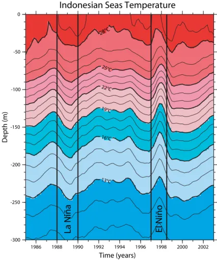
to 135°E and 12°S to 2°N Indonesian seas region and constructing a single time-depth section of temperature (Fig- ure 2). Ocean temperatures throughout the Indonesian seas (and the western Pacifi c Ocean) are cooler during El Niño years and warmer during La Niña years throughout the water column, with a maximum signal around 150-m

13°C 16°C 19°C 22°C 25°C 28°C

-300 -250 -200 -150 -100 -50 0

Depth (m)

1986 1988 1990 1992 1994 1996 1998 2000 2002

Time (years)

El Niño

La Niña

Indonesian Seas Temperature

Figure 2. Th e temperature time-depth section averaged over the 114°E to 135°E and 12°S to 2°N Indonesian seas region. ENSO variability is easily observed from the ocean surface down to the bottom of the XBT profi les

~760 m; this section only shows the upper 300 m of the water column in order to expand the mid-thermocline levels, which have the largest ENSO signal at ~150 m. Ocean temperatures throughout the Indonesian seas (and the western Pacifi c Ocean) are cooler during El Niño years and warmer dur- ing La Niña years; for example, in this section at 150 m, they attain tempera- tures ~1.5°C cooler than usual during the El Niño of 1997–1998 when the thermocline shallows and temperatures ~1.25°C warmer than usual during the La Niña of 1988–1989 when the thermocline deepens. Th e data are smoothed by a 20-m vertical fi lter and then a 1-yr horizontal fi lter.

Oceanography

Figure 3. Indonesian seas temperature and fi nestructure profi les contrasting the active Li- famatola Strait with the relatively quiescent Timor Sea. Th e Lifamatola Strait XBT tempera- ture profi le (a) reveals considerable structure at all depths and vertical scales. In contrast, the Timor Sea XBT temperature profi le (c) is relatively smooth at all depths. Regions with more fi nestructure may have more mixing. To quantify the fi nestructure observed in a XBT temperature profi le, the magnitude of the isotherm vertical displacements (in meters) are determined relative to the profi le smoothed by a 10-m block running mean. Calculated in this way, the fi nestructure variability of the Lifamatola Strait profi le (b) is large, with a 50 to 300 m depth average of 3.4 m, refl ecting the considerable vertical temperature structure observed in the temperature profi le. In contrast, the Timor Sea fi nestructure variability (d) is smaller, with a 50 to 300 m depth average of only 0.7 m, refl ecting the smoother tempera- ture profi le. Th e 50 m running block average of the fi nestructure is shown in blue.

depth. At 150 m, during the El Niño of 1997–1998, the temperatures are ~1.5°C cooler than usual when the thermo- cline shallows; during the La Niña of 1988–1989, the temperatures are ~1.5°C warmer than usual when the thermo- cline deepens.

Visually examining two temperature profi les reveals the fi nestructure and how

it may vary. A Lifamatola Strait tempera- ture profi le (Figure 3a) reveals consider- able temperature structure at a range of vertical scales from 2–100 m throughout the profi le; for example, between 50 and 100 m, there is a distinct 25°C, 50 m ver- tical step feature in addition to nearby smaller-scale bumps and wiggles in the profi le. In contrast, a relatively quiescent

Timor Sea temperature profi le (Figure 3c) is relatively smooth throughout. To quantify the fi nestructure observed in an XBT temperature profi le, we determined the magnitudes of the isotherm vertical displacements (in meters) relative to the profi le smoothed by a 10-m block run- ning mean. The focus is on fi nestructure at 2 to 10 m scales to avoid introducing biases from larger-scale circulation-relat- ed changes in the thermocline. Calculated in this way, the fi nestructure variability in the Lifamatola Strait profi le (Figure 3b) is large, with a 50 to 300 m depth aver- age of 3.4 m, refl ecting the considerable vertical temperature structure observed in the temperature profi le. In contrast, the Timor Sea fi nestructure variability (Figure 3d) is smaller, with a 50 to 300 m depth average of only 0.7 m, refl ecting the smoother temperature profi le.

To assess the geographic variability, we temporally averaged all 18 years of fi n- estructure results between 100 and 300 m depths and plotted them on the XBT transect map (Figure 1). The fi nestruc- ture is generally largest near topography (e.g., near coastlines, over shallow shelves, and within straits). Two notable regions are the Lifamatola Strait near 126°E, 2°S, which has average fi nestructure values greater than 1.5 m despite being within a deep and broad strait, and the Ombai Strait near 125°E, 8°S, which is also with- in a deep strait and has the largest aver- age fi nestructure values (greater than 2.0 m). When all these data are compiled as a function of distance to the nearest 100-m topography (not shown), a clear relation is evident; the highest fi nestructure val- ues are adjacent to topography and drop off smoothly with distance.

To assess the temporal variability, we spatially averaged all the fi nestructure

0 100 200 300 400 500 600 700

Depth (m)

6 9 12 15 18 21 24 27 30

Temperature (C) -- lots of stru

cture -- step 126.4E, -2.2S

Lifamatola Strait

a) b)

Temperature and Finestructure Profiles

0 100 200 300 400 500 600 700

0 5 10 15 20

Finestructure (m)

0 100 200 300 400 500 600 700

Depth (m)

6 9 12 15 18 21 24 27 30

Temperature (C) -- smoother -- 129.6E, -8.8S

Timor Sea

c) d)

0 100 200 300 400 500 600 700

0 5 10 15 20

Finestructure (m)

Oceanography

b) Finestructure (m) at 30 m

c) Finestructure (m) at 550 m

d) Niño 3

Indonesian Seas Time Series

16 18 20

1986 1989 1992 1995 1998 2001

MIN

MAX

3 4 5 6

1986 1989 1992 1995 1998 2001

MIN

MAX

4 5 6

1986 1989 1992 1995 1998 2001

MIN MAX

-2 0 2

1986 1989 1992 1995 1998 2001

La Niña El Niño

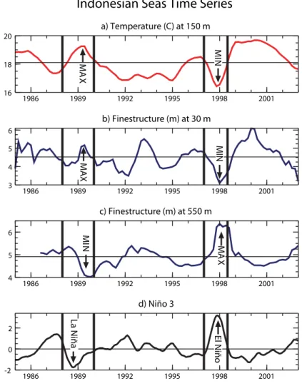
results into single time series. Using ex- amples highlighting different depths of the water column, the time series (Figure 4) of temperature at 150 m (a), fi nestruc- ture at 30 m (b), and fi nestructure at 550 m (c) all reveal ENSO variability when visually compared to the Niño 3 index (d). During the El Niño of 1997–1998, temperatures are cooler throughout the water column (Figure 2) and the 150- m mid-thermocline temperature is 8 percent cooler than average (Figure 4a).

However, the fi nestructure is 33 percent less than average at 30 m in the upper thermocline (Figure 4b), but 29 per- cent greater than average at 550 m in the lower thermocline (Figure 4c). This result can be explained by the increased (decreased) vertical temperature stratifi - cation in the upper 100 m (below 100 m) during an El Niño (not shown). There is also considerable monsoonal variability (not shown) in the fi nestructure, with much higher values in the upper 100 m during the strong June, July, and August monsoonal winds. These fi nestructure results can be used to put vertical mixing estimates into a geographic and temporal framework within the Indonesian seas.

ACKNOWLED GE MENTS

This project was supported by the Offi ce of Naval Research, NOOO14-03-1-0423.

Lamont-Doherty Earth Observatory con- tribution number 6820. Earth & Space Research contribution number 83.

REFERENCE S

Alford, M., M. Gregg, and M. Ilyas. 1999. Diapyc- nal mixing in the Banda Sea: Results of the fi rst microstructure measurements in the Indone- sian throughfl ow. Geophysical Research Letters 26:2,741–2,744.

Bray, N.A., S. Hautala, J. Chong, and J. Pariwono.

1996. Large-scale sea level, thermocline, and wind variations in the Indonesian through-

fl ow region. Journal of Geophysical Research 101:12,239–12,254.

Ffi eld, A., and A. Gordon. 1996. Tidal mixing signa- tures in the Indonesian Seas. Journal of Physical Oceanography 26:1,924–1,937.

Ffi eld, A., K. Vranes, A.L. Gordon, R.D. Susanto, and S.L. Garzoli. 2000. Temperature Variability within Makassar Strait. Geophysical Research Letters 27:237–240.

Finnigan, T.D., D.S. Luther, and R. Lukas. 2002.

Observations of Enhanced Diapycnal Mixing near the Hawaiian Ridge. Journal of Physical Oceanography 32:2,988–3,002.

Hatayama, T. 2004. Transformation of the Indone- sian throughfl ow water by vertical mixing and

its relation to tidally generated internal waves.

Journal of Oceanography 60:569–585.

Hautala, S., J. Reid, and N. Bray. 1996. The distribu- tion and mixing of Pacifi c water masses in the Indonesian seas. Journal of Geophysical Research 101:12,375–12,389.

Sprintall, J., J.T. Potemra, S.L. Hautala, N.A. Bray, and W.W. Pandoe. 2003. Temperature and salinity variability in the exit passages of the Indonesian throughfl ow. Deep-Sea Research II 50:2,183–2,204.

Wijffels, S., and G. Meyers. 2004. An Intersection of oceanic waveguides: Variability in the Indo- nesian throughfl ow region. Journal of Physical Oceanography 34:1,232–1,253.

Figure 4. Time series of temperature at 150 m (a), fi nestructure at 30 m (b), and fi nestructure at 550 m (c) averaged over the 114°E to 135°E and 12°S to 2°N Indone- sian seas region. Th e Niño 3 index is shown for comparison in (d). All the variables reveal ENSO variability. During the El Niño of 1997–1998, the temperature at 150 m is cooler than average (a), as are all the temperatures throughout the water column (Figure 2). However, the fi nestructure is less than average at 30 m in the upper water column (b), but greater than average at 550 m in the lower water column (c).