RIMS-1697
The perturbative invariants of rational homology 3-spheres can be recovered from the LMO invariant
By
Takahito KURIYA, Thang T. Q. Le, Tomotada OHTSUKI
May 2010
R ESEARCH I NSTITUTE FOR M ATHEMATICAL S CIENCES
The perturbative invariants of rational homology 3-spheres can be recovered from the LMO invariant
Takahito Kuriya, Thang T. Q. Le, Tomotada Ohtsuki
Abstract
We show that the perturbativeginvariant of rational homology 3-spheres can be recovered from the LMO invariant for any simple Lie algebra g, i.e., the LMO invariant is universal among the perturbative invariants. This universality was conjectured in [25]. Since the perturbative invariants dominate the quantum invariants of integral homology 3-spheres [13, 14, 15], this implies that the LMO invariant dominates the quantum invariants of integral homology 3-spheres.
1 Introduction
In the late 1980s, Witten [33] proposed topological invariants of a closed 3-manifold M for a simple compact Lie group G, which is formally presented by a path integral whose Lagrangian is the Chern-Simons functional of G connections on M. There are two approaches to obtain mathematically rigorous information from a path integral: the operator formalism and the perturbative expansion. Motivated by the operator formalism of the Chern-Simons path integral, Reshetikhin and Turaev [31] gave the first rigorous mathematical construction of quantum invariants of 3-manifolds, and, after that, rigorous constructions of quantum invariants of 3-manifolds were obtained by various approaches.
WhenM is obtained fromS3 by surgery along a framed knotK, the quantumGinvariant τrG(M) of M is defined to be a linear sum of the quantum (g, Vλ) invariant Qg,Vλ(K) of K at anrth root of unity, whereg is the Lie algebra of G, and Vλ denotes the irreducible representation of g whose highest weight is λ. On the other hand, the perturbative expansion of the Chern-Simons path integral suggests that we can obtain the perturbative g invariant (a power series) when we fix g, and obtain the LMO invariant (an infinite linear sum of trivalent graphs) when we make the perturbative expansion without fixing g. As a mathematical construction, we can define the perturbativeginvariantτg(M) of a rational homology 3-sphereM by arithmetic perturbative expansion ofτrP G(M) asr→ ∞ [27, 32, 23], whereP Gdenotes the quotient ofGby its center. Further, we can present the LMO invariant ˆZLMO(M) [25] of a rational homology 3-sphere M by the Aarhus integral [5]. It was conjectured [25] that the perturbative g invariant can be recovered from the LMO invariant by the weight system ˆWg for any simple Lie algebra g. In the sl2 case, this has been shown in [28]. See Figures 1 and 2, for these invariants and relations among them.
The aim of this paper is to show the following theorem.
Chern-Simons path integral
¡¡
¡¡
¡¡ ª Operator formalism
Quantum invariantτrG(M)
@@
@ Perturbative expansion
¡¡
¡ ª
Fixingg Without fixing g Perturbative
invariantτg(M) HHHHHj
The LMO
invariant ˆZLMO(M) Figure 1: Physical background
τg(M) ≈ Wˆg( ˆZLMO(M))
´´´´3
Arithmetic perturbative expansion
Quantum
invariantτrP G(M)
XX XX XX y
Weight system ˆWg
The LMO
invariant ˆZLMO(M)
QQ QQ
Gaussian sumk
on a set⊂h∗ ppppp ppp ppp pppppp ppp ppp
ppppppppppppppppppppppp
Quantum invariant
Qg,Vλ(K) XyXXXXX
Weight
system ˆWg ¢¢¢¢¢¢¸
Aarhus integral
The Kontsevich invariantZ(K) Figure 2: Mathematical construction
Theorem 1.1 (see [3, 21]1). Let g be any simple Lie algebra. Then, for any rational homology 3-sphere M,
Wˆg¡ZˆLMO(M)¢
= |H1(M;Z)|(dimg−rankg)/2τg(M),
where |H1(M;Z)| denotes the cardinality of the first homology group H1(M;Z) of M. We give two proofs of the theorem: a geometric proof (Sections 4.1 and 5.2) and an algebraic proof (Sections 4.2 and 5.1). The theorem implies that the LMO invariant dominates the perturbative invariants. Further, since the perturbative invariants domi- nate the quantum Witten-Reshetikhin-Turaev invariants of integral homology 3-spheres [13, 14, 15], it follows from the theorem that the LMO invariant dominates the quantum invariants of integral homology 3-spheres.2
Let us explain a sketch of the proof when M is obtained by surgery on a knot. The LMO invariant ˆZLMO(M) can be presented by the Aarhus integral [5]. It is shown from this presentation that the image ˆWg¡ZˆLMO(M)¢
can be presented by an integral of Gauss type over the dual g∗, or alternatively by an expansion given in terms of the Laplacian
∆g∗ of g∗. On the other hand, as we explain in Section 6.2, the perturbative invariant τg(M) is presented by a Gaussian integral overh∗, whereh is a Cartan subalgebra ofg, or
1It was announced in [3] that the perturbativeginvariant can be recovered from the LMO invariant. However, their proof is not published yet. The first author [21] showed a proof, but his proof is partially incomplete. The aim of this paper is to show a complete proof of the theorem.
2For rational homology 3-spheres, it is known [9] that the quantum WRT invariantτrSO(3)(M), at roots of unity of order co-prime to the order of the first homology group, can be obtained from the perturbative invariant τsl2(M). Hence, the LMO invariant ˆZLMO(M) dominatesτrSO(3)(M) for those roots of unity.
alternatively by an expansion given in terms of the Laplacian ∆h∗ofh∗. We then show that Wˆg¡ZˆLMO(M)¢
= τg(M) by establishing a result relating integrals over g∗ and integrals over h∗, similar to the well known Weyl reduction integration formula. Alternatively, we show ˆWg¡ZˆLMO(M)¢
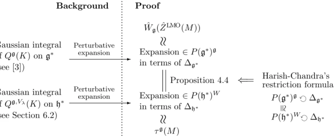
= τg(M) by using Harish-Chandra restriction theorem that relates the Laplacian ∆g∗ ong∗ to the Laplacian ∆h∗ onh∗. For a sketch of the algebraic proof, see also Figure 3.
Wˆg( ˆZLMO(M))
≈
τg(M
≈
) pppppppppppp pppppp pppppp pppppp pppppp pppppp pppppp pppp
Background Proof
Gaussian integral ofQg(K) ong∗ (see [3])
Gaussian integral ofQg,Vλ(K) onh∗ (see Section 6.2)
-
-
Perturbative expansion
Perturbative expansion
Expansion∈P(g∗)g in terms of ∆g∗
Expansion∈P(h∗)W in terms of ∆h∗
Proposition 4.4 ⇐= Harish-Chandra’s restriction formula
P(g=∼∗)g ª ∆g∗
P(h∗)W ª ∆h∗
Figure 3: Sketch of the algebraic proof of Theorem 1.1, whenM is obtained fromS3by surgery along a framed knotK
In case when M is obtained by surgery on a link we also present two proofs. The first one is more algebraic. We reduce the theorem to the case of surgery on knots by using the fact that the operators involved are invariant under the action of g. The other proof has quite a different flavor. We show that two multiplicative finite type invariants of rational homology spheres are the same if they agree on the set of rational homology spheres obtained by surgery on knots (for finer results see Theorem 5.4). This result is also interesting by itself. The theorem then follows, since both ˆWg
¡ZˆLMO(M)¢
andτg(M), up to any degree, are finite type. This part relates the paper to the origin of the theory:
The discovery of the perturbative invariant of homology 3-spheres for SO(3) case [27]
leads the third author to define finite type invariants of 3-manifolds.
The paper is organized, as follows. In Section 2, we review definitions of terminologies, and show some properties of Jacobi diagrams. In Section 3, we present the proof of the main theorem, based on results proved later. We consider the knot case in Section 4 and the link case in Section 5. In Section 6, we discuss how the perturbative invariant can be obtained as an asymptotic expansion of the Witten-Reshetikhin-Turaev invariant, and give a proof that our formula of the perturbative invariant is coincident with that given in [23]. We also show that finite parts of the perturbative invariant τg are of finite type.
The third author would like to thank Susumu Ariki for pointing out Harish-Chandra’s restriction formula when he tried to prove Proposition 4.4 in the sl3 case. The authors would like to thank Dror Bar-Natan, Kazuo Habiro, Andrew Kricker, Lev Rozansky, Toshie Takata and Dylan Thurston for valuable comments and suggestions on early ver- sions of the paper.
2 Preliminaries
In this section, we recall basic facts about Lie algebras in Section 2.1 and theory of the Kontsevich invariant in Section 2.3. We show some facts about Laplacian operators in Euclidean spaces in Section 2.2, and present the LMO invariant in Section 2.4.
2.1 Lie algebra
In this paper, Gis a compact connected simple Lie group, g its Lie algebra andh a fixed Cartan subalgebra of g. Up to scalar multiplication, there is a unique Ad-invariant inner product on g. The complexification gC of g can be presented as gC =g+√
−1g. Then hC =h+√
−1h is a Cartan subalgebra ofgC.
There is a root system ΦC ⊂(hC)∗ of the pair (gC,hC). It is known that ΦC, as well as the weights ofg-modules, are purely imaginary,i.e., ΦC⊂(√
−1h)∗ ≡√
−1h∗. Following the common convention in Lie algebra theory (see e.g. [16]), we call β ∈ h∗ a real root (resp. a real weight of a g-module) if √
−1β is a root (resp. a weight of the g-module).
We normalize the invariant inner product so that the square length of every short root is 2. We denote by W the Weyl group, Φ+ the set of positive real roots of g, and ρ the half-sum of positive real roots. Let φ+ be the number of positive roots of g. One has φ+ = (dimg− dimh)/2 = (dimg− rankg)/2. We denote by Vλ the irreducible representation of g whose highest weight is√
−1λ.
Let S(g) and U(g) be respectively the symmetric tensor algebra and the universal enveloping algebra of g. One can naturally identify S(g) with P(g∗), the algebra of polynomial functions on g∗. Throughout the paper, ~ is a formal parameter, and q = e~∈R[[~]]. One considers S(g)[[~]] as a ring of functions on g∗ with values in R[[~]].
The following W-skew-invariant functions D is important to us:
D(λ) := Y
α∈Φ+
(λ, α) (ρ, α).
When λ−ρ is a dominant real weight, D(λ) is the dimension of Vλ−ρ.
We identify h∗ with a subspace ofg∗ using the invariant inner product. For a function g ong∗, its restriction to h∗ will be denoted by P(g).
A source of function on h∗ is given by the enveloping algebraU(g). For g ∈U(g) we define a polynomial function, also denoted by g, on h∗ as follows. Suppose λ−ρ is a dominant real weight. One can take the trace TrVλ−ρ(g) of the action ofg in theg-module Vλ−ρ. It is known that there is a unique polynomial function, denoted by also byg, onh∗ such that g(λ) = TrVλ−ρ(g).
There is a vector space isomorphism Υg : S(g) → U(g), known as the Duflo-Kirillov map (see [7, 2, 8]). We can extend Υg multi-linearly to a vector space isomorphism Υg : S(g)⊗` → U(g)⊗`. When restricted to the g-invariant parts, Υg : S(g)g → U(g)g is an algebra isomorphism. Note that U(g)g is the center of the algebra U(g).
2.2 Laplacian and Gaussian integral on a Euclidean space
LetV be a Euclidean space. In our applications we will always haveV =gorV =hwith the Euclidean structure coming from the invariant inner product. As usual, one identifies the symmetric algebra S(V) with the polynomial function algebra P(V∗). The Laplacian
∆V, associated with the Euclidean structure ofV, acts on S(V) = P(V∗) and is defined by
∆V = X
i
∂x2i,
wherexi’s are coordinate functions with respect to an orthonormal basis ofV. It is known that for x, y ∈V, 12∆V(xy) = (x, y), the inner product ofx and y.
Let~be a formal parameter. For a non-zero real numberf let us consider the following operator EV(f) :S(V) =P(V∗)→R[1/~] expressed through an exponent of the Laplacian and the evaluation at 0:
EV(f)(g) = exp µ
− ∆ 2f~
¶ (g)¯¯
x=0 ∈R[1/~].
Because ∆V is a second order differential operator, it is easy to see that if g is a homoge- neous polynomial, then
EV(f)(g) = (
0 if deg(g) is odd,
scalar
~deg(g)/2 if deg(g) is even. (1)
Adjoining ~, we get an extension EV(f) : S(V)((~)) =P(V∗)((~))→R((~)) as follows. If g =P∞
n=−∞gn~n with gn∈S(V), then EV(f)(g) =X
n
EV(f)(gn)~n ∈R((~)).
There is a generalization to the multi-variable case. Suppose f := (f1, . . . , f`) is an
`-tuple of non-zero real numbers and g1⊗ · · · ⊗g` ∈S(V)⊗`, then we define EV(f)(g1⊗ · · · ⊗g`) =
Y` j=1
EV(fj)(gj).
Formally we can put EV(f) = N
jEV(fj). Again there is an obvious extension EV(f) : S(V)⊗`((~))→R((~)).
2.3 Jacobi diagrams, weight systems, and the Kontsevich invariant
In this section, we review Jacobi diagrams, weight systems, and the Kontsevich invariant of framed string links. For details see e.g. [29].
A uni-trivalent graph is a graph every vertex of which is either univalent or trivalent.
A uni-trivalent graph is vertex-oriented if at each trivalent vertex a cyclic order of edges is fixed. For a 1-manifold Y, a Jacobi diagram on Y is the manifold Y together with a
vertex oriented uni-trivalent graph such that univalent vertices of the graph are distinct points on Y. In figures we draw Y by thick lines and the uni-trivalent graphs by thin lines, in such a way that each trivalent vertex is vertex-oriented in the counterclockwise order. We define the degree of a Jacobi diagram to be half the number of univalent and trivalent vertices of the uni-trivalent graph of the Jacobi diagram. We denote byA(Y) the quotient vector space spanned by Jacobi diagrams onY subject to the following relations, called the AS, IHX, and STU relations respectively,
=− , = − , = − .
For S = {x1,· · · , x`}, a Jacobi diagram on S is a vertex-oriented uni-trivalent graph whose univalent vertices are labeled by elements of S. We denote byA(∗S) the quotient vector space spanned by Jacobi diagrams on S subject to the AS and IHX relations. In particular, when S consists of a single element, we denote A(∗S) by A(∗). A(∅) and A(∗S) form algebras with respect to the disjoint union of Jacobi diagrams, and A(t`↓) forms an algebra with respect to the vertical composition of copies oft`↓.
We briefly review weight systems; for details, see [1, 29]. We define the weight system Wg(D) of a Jacobi diagram D by “substituting” g into D, i.e., putting D in a plane, Wg(D) is defined to be the composition of intertwiners, each of which is given at each local part ofD as follows.
RxB g⊗g
g⊗g x
R
xg
[·,·]
g⊗g
Here, the first map is the invariant form of g, and the second map is the map taking 1 to P
iXi ⊗Xi, where {Xi}i∈I is an orthonormal basis of g with respect to the invariant form, and the third map is the Lie bracket of g. For D1 ∈ A(∗) and D2 ∈ A(↓), we have the following intertwiners as the compositions of the above maps, and we can define Wg(D1)∈S(g) andWg(D2)∈U(g) as the images of 1 by these maps.
D1
S(g)x
R
D2
U(g) x
R In a similar way, we can also define Wg : A(t` ↓) → ¡
U(g)⊗`¢g
and Wg : A(∗S) →
¡S(g)⊗`¢g
; they are algebra homomorphisms. Note that there is a standard degree on the polynomial algebra S(g)⊗` which carries over to U(g)⊗` by the Poincare-Birkhoff-Witt isomorphism. If D is a diagram with k univalent vertices, then Wg(D) has degree ≤ k.
The weight system WgC is defined in the same way. Since WgC = Wg by definition, we denoteWg
C byWg. Further, we define ˆWgby ˆWg(D) =Wg(D)~d for a Jacobi diagramD of degree d.
There is a formal Duflo-Kirillov algebra isomorphism Υ : A(∗) → A(↓) (see [2, 8]).
The obvious multi-linearly extension Υ : A({x1, . . . , x`}) → A(t` ↓) is not an algebra
isomorphism, but a vector space isomorphism. The following diagram is commutative [2, Theorem 3].
A(∗) −−−→Wˆg S(g)g[[~]] P(g∗)g[[~]]
Υ
y∼= Υgy∼= ∼=yP A(↓) −−−→
Wˆg
U(g)g[[~]] −−−→∼=
ψg
P(h∗)W[[~]]
(2)
Here, P(h∗)W denotes the algebra of W-invariant polynomial functions on h∗. Υ denotes the Duflo-Kirillov isomorphism. ψgdenotes the Harish-Chandra isomorphism; forλ∈h∗, ψg(z)(λ) is defined to be the scalar by which z ∈ U(g)g acts on the irreducible represen- tation of g whose highest weight is λ−ρ. In other words, ψg(z)(λ) = z(λ)/D(λ). P is the restriction map from g∗ toh∗.
A string link is an embedding ϕ of ` copies of the unit interval, [0,1]× {1}, · · ·, [0,1]× {`}, into [0,1]×C, so that ϕ¡
(ε, j)¢
= (ε, j) for all ε ∈ {0,1} and 1 ≤ j ≤ `.
We obtain a link from a string link by closing each component of t`↓. A (string) link is called algebraically split if the linking number of each pair of components is 0.
The Kontsevich invariant Z(T) [20, 24] of an `-component framed string link T is defined to be in A(t` ↓); for its construction, see, e.g., [24, 29]. Let ν = Z(U), the Kontsevich invariant of the unknot U with framing 0; the exact value of ν is calculated in [8]. Using the Poincare-Birkhoff-Witt isomorphism A(S1) ∼= A(↓) (see [1]), we will considerν as an element in A(↓).
Let ∆(`) : A(↓) → A(t` ↓) be the cabling operation which replaces an arrow by ` parallel copies (see e.g. [24, Section 1]). The modification ˇZ(T) of Z(T) used in the definition of the LMO invariant is
Z(Tˇ ) :=ν⊗` ¡
∆`(ν)¢
Z(T).
Applying Υ−1 followed by the weight map, we define the following element:
Qˇg(T) = ˆWg
³
Υ−1¡Z(Tˇ )¢´
∈¡
S(g)⊗`¢g
[[~]]. (3)
2.4 Presentations of the LMO invariant
In this section, we recall and modify a formula of the LMO invariant [25] of a rational homology 3-sphere M using the Aarhus integral [5] for the case when M is obtained by surgery along an algebraically split link.
Suppose T is an algebraically split `-component string link with 0 framing on each component, and L is its closure. Suppose the components of T are ordered. Let f = (f1, . . . , f`) be an`-tuple of `non-zero integers, andM be the rational homology 3-sphere obtained by surgery on L with framing f1, . . . , f`.
Let θ ∈ A(∅) be the following Jacobi diagram
θ = ∈ A(∅). (4)
Define
I(T,f) := exp
³− P
jfj
48 θ´* Y
j
exp
³− 1 2fj
∂xj ∂xj´ , ¡
Υ−1¢Z(Tˇ ) +
∈ A(∅). (5) Here, for a Jacobi diagramD1 whose univalent vertices are labeled by∂xj’s and a Jacobi diagram D2 whose univalent vertices are labeled by xj’s, we define the bracket by
hD1, D2i =
³ the sum of all ways of gluing the ∂xj-labeled univalent vertices of D1 to the xj-labeled univalent vertices ofD2 for each j
´∈ A(∅),
if the number of∂xj-labeled univalent vertices ofD1 are equal to the number ofxj-labeled univalent vertices of D2 for each j, and put hD1, D2i= 0 otherwise. In particular, when T =↓ is the trivial string link, one has
I(↓,±1) = exp
³∓ 1 48θ
´*
exp
³∓ 1 2
∂x ∂x´
, Υ−1(ν2) +
∈ A(∅), Then, the LMO invariant of M is presented by3
ZˆLMO(M) = I(T,f) Q`
j=1I(↓,sign(fj)) ∈ A(∅). (6) We remark that the presentation (6) is obtained from [6, Theorem 6], noting that (with notations from [6])
˚A0(L) = Z ³ Y
j
Υ−xj1´¡Z(L)ˇ ¢ dX,
³ Y
j
Υ−xj1´¡Z(L)ˇ ¢
= ³ Y
j
Υ−xj1´¡Zˇ(T)¢ exp
³− P
jfj 48 θ´ Y
j
exp
³fj 2 xj xj
´ ,
which are obtained from Lemma 3.8 and Corollaries 3.11 and 3.12 of [6].
3 Proof of the main theorem
In this section we show the proof of the main theorem in Section 3.2 based on results proved in later sections.
3.1 Comparing the LMO invariant and the perturbative invariant
We again assume M, L, T,f the same as in Section 2.4. Recall that in (3) we defined Qˇg(T)∈(S(g)⊗`)g[[~]].
3The bracket of this presentation is called the Aarhus “integral”, since its corresponding Lie algebra version is actually an integral on (g∗)⊕`[3].
Proposition 3.1. Assume the above notations.
a) The LMO invariant of M, after applied by the weight map, has the following presen- tation
Wˆg( ˆZLMO(M)) = I1(T,f) Q`
j=1I1(↓,sign(fj)), (7) where
I1(T,f) = Ã `
Y
j=1
q−fj|ρ|2/2
! Eg(f)
¡Qˇg(T)¢ .
b) The perturbative invariant has the following presentation τg(M) = I2(T,f)
Q`
j=1I2(↓,sign(fj)), (8) where
I2(T,f) = Ã `
Y
j=1
q−fj|ρ|2/2
! Eh(f)
¡D⊗`Υg( ˇQg(T))¢ .
Proof. Apply the algebra map ˆWgto (6),
Wˆg( ˆZLMO(M)) = Wˆg(I(T,f)) Q`
j=1Wˆg¡
I(↓,sign(fj))¢. Using Lemmas 3.3, 3.4 and the definition of I(T,f) in (5) we get
Wˆg(I(T,f)) =I1(T,f),
which proves part (a) of the proposition. Part (b) will be proved in Section 6.3.
To prove the main theorem one needs to understand the relation betweenEg(f) andEh(f). We will prove the following proposition in Sections 4 and 5.
Proposition 3.2. There is a non-zero constant cg such that for g ∈ (S(g)⊗`)g[[~]] and any `-tuple f = (f1, . . . , f`) of non-zero integers one has
Eg(f)(g) = Ã `
Y
j=1
(−2fj~)φ+cg
! Eh(f)¡
D⊗`Υg(g)¢
. (9)
3.2 Proof of Main Theorem
Now we can prove Theorem 1.1. First we assume that M can be obtained by surgery along an algebraically split link L. We assumeT,f as in Section 2.4. One has
I1(T,f) = Ã `
Y
j=1
q−fj|ρ|2/2
! Eg(f)
¡Qˇg(T)¢
= Ã `
Y
j=1
q−fj|ρ|2/2
! Ã ` Y
j=1
(−2fj~)φ+cg
! Eh(f)
¡D⊗`Υg¡Qˇg(T)¢¢
= Ã `
Y
j=1
(−2fj~)φ+cg
!
I2(T,f), (10)
where the second equality follows from Proposition 3.2 since ˇQg(T) ∈ (S(g)⊗`)g[[~]]. In particular, applying (10) for (T,f) = (↓,sign(fj)), then taking the product when j runs from 1 to `, one has
Y` j=1
I1(↓,sign(fj)) = Y` j=1
³¡−2 sign(fj)~¢φ+
cgI2¡
↓,sign(fj)¢´
, (11)
Dividing (10) by (11) and using Proposition 3.1, we have Wˆg( ˆZLMO(M)) =
Y` j=1
|fj|φ+τg(M)
=|H1(M,Z)|τg(M).
This completes the proof the Theorem 1.1 for the case whenM can be obtained by surgery along an algebraically split link.
Let us consider the general case, when M is an arbitrary rational homology 3-sphere.
It is known [27] that, there exist some lens spaces L(m1,1), · · ·, L(mN,1) such that the connected sum M#L(m1,1)#· · ·#L(mN,1) can be obtained from S3 by surgery along some algebraically split framed link. Since the LMO invariant and the perturbative invariant are multiplicative with respect to the connected sum, it follows from the above case that
Wˆg¡ZˆLMO(M)¢
·Y
i
Wˆg
³ZˆLMO¡
L(mi,1)¢´
= |H1(M;Z)|φ+τg(M)·Y
i
³¯¯H1¡
L(mi,1);Z¢¯¯φ+τg¡
L(mi,1)¢´
.
In particular, since the lens space L(mi,1) can be obtained from S3 by surgery along a framed knot, it also follows from the above case that
Wˆg
³ZˆLMO¡
L(mi,1)¢´
= ¯¯H1¡
L(mi,1);Z¢¯¯φ+τg¡
L(mi,1)¢ .
Further, since the leading coefficient of the LMO invariant is 1, the value of the above formula is non-zero. Therefore, as the quotient of the above two formulas, we obtain the required formula. This completes the proof of Theorem 1.1 in the general case.
3.3 Some lemmas on weights of Jacobi diagrams
In this section, we show some lemmas on Jacobi diagrams which are used in the proof of Proposition 3.1.
Lemma 3.3. For a Jacobi diagram D∈ A(∗) and a non-zero real number f, Wˆg
³D
exp¡−1 2f
∂x ∂x¢ , D
E´
= Eg(f)
¡Wˆg(D)¢ .
Proof. The bracket can be presented in terms of differentials as explained in [3, Appendix].
We verify this for the required formula concretely.
By expanding the exponential, it is sufficient to show that Wg³D¡∂x ∂x¢d
, D E´
= ∆dg∗
¡Wg(D)¢¯¯
Xi=0. (12)
Since both sides are equal to 0 unless D has 2d legs, we can assume that D has 2d legs.
When d= 1, (12) is shown by Wg
³D∂x ∂x , D
E´
= Wg
³
2 D
´
= 2B¡
Wg(D)¢
= ∆g∗¡
Wg(D)¢ , where B is the invariant form. When d = 2, putting Wg(D) = P
kY1,kY2,kY3,kY4,k for Yi,j ∈g, (12) is shown by
Wg³D¡∂x ∂x¢2
, D E´
= X
τ
Wg
³ τ
D
´
= X
τ,k
B(Yτ(1),k, Yτ(2),k)B(Yτ(3),k, Yτ(4),k)
= X
τ,i,j,k
∂Xi(Yτ(1),k)∂Xi(Yτ(2),k)∂Xj(Yτ(3),k)∂Xj(Yτ(4),k) = ∆2g∗
¡Wg(D)¢ ,
where the sum of τ runs over all permutations on {1,2,3,4}. For a general d, we can show (12) in the same way as above.
Lemma 3.4 ([21]). For the Jacobi diagram θ given in (4), Wg(θ) = 24|ρ|2, where ρ is the half-sum of positive roots.
Proof. It is shown from the definition of the weight system (see, e.g., [29]) that Wg¡ ¢
= CadWg¡ ¢
and Wg¡ ¢
= dimg,
whereCad denotes the eigenvalue of the Casimir element on the adjoint representation of g. Hence, Wg(θ) =Caddimg.
It is known that, Cad = (δ, δ + 2ρ), where δ is the highest weight of the adjoint representation, which is longest positive root. In our normalization of the inner product, (δ, δ) = 2d and (δ, ρ) =dh∨−d, where h∨ denotes the dual Coxeter number ofg and d is the maximal absolute value of the off-diagonal entries of the Cartan matrix. Therefore, Wg(θ) = 2dh∨dimg.
Further, it is known [10, 47.11] (adjusted to our normalization of the inner product) that 2dh∨dimg= 24|ρ|2. Hence, we obtain the required formula.
4 The knot case
The aim of this section is to prove Proposition 3.2 for the case ` = 1. We call this the knot case, since Proposition 3.2 with ` = 1 is enough to prove the main theorem for the case whenM is obtained by surgery on a knot. We show a geometric proof in Section 4.1 and an algebraic proof in Section 4.2.
4.1 Geometric approach
Geometric proof of Proposition 3.2 in the knot case. Since`= 1,g ∈S(g)g[[~]]. Without loss of generality, one can assume that g ∈S(g)g. We will write f1 =f. Note that g is a function ong; it’s restriction on h∗ is denoted byP(g). On the other hand, Υg(g)∈U(g) defines a function onh∗, see Section 2.1. From the commutativity of Diagram 2, we have that, as functions on h∗,
Υg(g) = D P(g). (13)
The left-hand side of (9) is Eg(f)(g), which, by Proposition 4.1, can be expressed by an integral:
LHS of (9) =Eg(f)(g) = 1 (4π)dimg/2
Z
g∗
e−|x|2/4g( x
√−2f~)dx
The integrand is invariant under the co-adjoint action. Hence, according to Proposition 4.3 below, one can reduce the integral to an integral over the Cartan subalgebra:
LHS of (9) = ˜cg (4π)dimg/2
Z
h∗
D2(x)e−|x|2/4P(g)
³ x
√−2f~
´
dx. (14) Here, ˜cg is a non-zero constant depending on the Lie algebra g only.
We turn to the right-hand side of (9). Using (13) one has RHS of (9) = cg(−2f~)φ+Eh(f)(D2P(g)).
Again using Proposition 4.1 we have
RHS of (9) =cg(−2f~) 1 (4π)dimh/2
Z
h∗
e−|x|2/4D2³ x
√−2f~
´ g
³ x
√−2f~
´
dx. (15) Because D2 is a homogeneous polynomial of degree 2φ+, one has
D2(x) = (−2f~)φ+D2³ x
√−2f~
´ . Withcg= c˜g
(4π)φ+, from (14) and (15) we see that
LHS of (9) = RHS of (9).
4.1.1 Gaussian integral and EV(f)
SupposeV is a Euclidean space andf a non-zero number. The following lemma says that the operator EV(f) can be expressed by an integral.
Lemma 4.1. Supposeg ∈S(V)((h)), considered as a function onV∗ with values in R((h)).
Then
EV(f)(g) = 1 (4π)dimV /2
Z
V∗
e−|x|2/4g
³ x
√−2f~
´
dx. (16)
Remark 4.2. Here, g
³√x
−2f~
´
is the function on V∗ with values in C((~1/2)) defined as follows. If g is of the form g =zd where z ∈V, then
g
³ x
√−2f~
´
:=g(x)
³ (p
−2f~)−d
´ .
The square root in the right-hand side does not really appear, since if dis odd, then both sides of (16) are 0.
Proof. We can assume that g ∈ S(V). Every polynomial is a sum of powers of linear polynomials. Since both sides of (16) depend linearly on g, we can assume that g is a power of a linear polynomial. By changing coordinates one can assume that g = xd1, wherex1 is the first of an orthonormal basisx1, . . . , xn ofV. The statement now reduces to the case when V is one-dimensional, which follows from a simple Gaussian integral calculation, see e.g. [7, Lemma 2.11].
4.1.2 Reduction from g∗ to h∗
Proposition 4.3. Suppose g is a G-invariant function on g∗. Then Z
g∗
g dx = ˜cg Z
h∗
D2P(g)dx
provided that both side converges absolutely. Here, c˜g is a non-zero constant depending only on g.
Proof. It is clear that if such ˜cg exists, then it is non-zero, since there are G-invariant functions g,e.g. g(x) = exp(−|x|2), for which the left-hand side is non-zero.
The co-adjoint action of G on g∗ is well-studied in the literature. A point x ∈ g∗ is regular if its orbit G·x is a submanifold of dimension dimg−dimh= 2φ+, the maximal possible dimension. It is known that the set of non regular points has measure 0. Every orbit has non-empty intersection with h∗, and if x is regular, thenG·x∩h∗ has exactly
|W| points. Since the functiong is constant on each orbit, we have Z
g∗
g(x)dx = 1
|W| Z
h∗
Vol(G·x)P(g)(x)dx.
The volume function is also well-known; it can be calculated, for example, from [7, Chapter 7]:
Vol(G·x) = ˜c0gD2(x) (17)
where ˜c0g is a constant. From (17) we can deduce the proposition, with ˜cg= ˜c0g/|W|. Here is a simple proof4 of (17). We will identify g with g∗ via the invariant inner product. LetH be the maximal abelian subgroup ofG whose Lie algebra ish. The space G/H is a homogeneousG-space. The tangent space of G/H atH can be identified with h⊥, with inner product induced from the invariant; from this we define a Riemannian metric on G/H. Whenx∈h is a regular, its stationary group is isomorphic to the torus H. The mapϕ :G/H →G·h, defined byg →g·xwith g ∈G, is a diffeomorphism. The tangent space of G·x at x can also be identified with the same h⊥ with the same inner product. It is easy to see that ϕ at H has derivative dϕH = −ad(x) : h⊥ → h⊥. Let us calculate the determinant ofdϕ. BecauseG/H isG-homogeneous andϕ isG-equivariant,
|det(dϕ)| is constant on G/H, hence |det(dϕ)| = |det(ad(x)|. To calculate |det(ad(x)|, it’s easier to use the complexification of the adjoint representation, since ad(x) is diagonal in the complexified representation. The complexifiedh⊥C has the standard Chevalley basis Eα, Fα, α∈Φ+ such that ad(x)Eα =i(x, α)Eα and ad(t)Fα =−i(x, α)Fα. It follows that
|dϕ|=Q
α∈Φ+|(x, α)|2. Hence
Vol(G·x) = Vol(G/H) Y
α∈Φ+
|(x, α)|2 = ˜c0gD2(x),
where ˜c0g= Vol(G/H)Q
α∈Φ+|(ρ, α)|2. 4.2 Algebraic approach
In this section, we show an algebraic proof of Proposition 3.2 in the knot case, i.e. the case ` = 1. We also verify some formulas of the proof in the sl2 case and in the sl3 case in Sections 4.2.1 and 4.2.2 respectively.
Algebraic proof of Proposition 3.2 in the knot case. Again we can assume thatg ∈S(g)g. By definition, the left-hand side of (9) is
Eg(f)(g) = exp¡
− 1
2f~∆g∗¢¡
g¢¯¯¯
x=0. By expanding the exponential,
LHS of (9) = X
d≥0
¡− 1 2f~
¢d 1
d!∆dg∗(gd), (18) where gd is the degree 2d part of g.
Let us turn to the right-hand side of (9). Recall that D has degree φ+. By (13) LHS of (9) = cg(−2f~)φ+Eh(f)(D2P(g))
= cg(−2f~)φ+ exp¡
− 1
2f~∆h∗¢¡
D2P(g)¢¯¯¯
x=0
4The authors thank A. Kirillov Jr. for supplying them the proof.
= cg(−2f~)φ+ X
d≥0
¡− 1 2f~
¢d+φ+ 1
(d+φ+)!∆d+φh∗ +¡
D2P(gd)¢
= cg X
d≥0
¡− 1 2f~
¢d 1
(d+φ+)!∆d+φh∗ +
¡D2P(gd)¢
. (19)
Comparing (18) and (19) by using Proposition 4.4 below, we have immediately LHS of (9) = RHS of (9).
This completes the algebraic proof of Proposition 3.2 in the knot case.
Proposition 4.4. For any homogeneous polynomial g ∈S(g)g of degree 2d, cg
d!∆dg∗(g) = 1
(d+φ+)!∆d+φh∗ +
¡D2P(g)¢ , where cg is a non-zero constant depending on g only.
Proof. Since the right hand side is not identically 0, if such acgexists, then it is non-zero.
We show that the identity of the proposition holds true if we takecg= ∆φh∗+
¡D2¢
/(φ+)!.
Since ∆dg∗(g) is a scalar, we have that D∆dg∗(g) =D P¡
∆dg∗(g)¢
= ∆dh∗
¡Dg¢ ,
where we obtain the second equality by applying Proposition 4.6 below repeatedly. Hence, substituting the above formula,
∆φh∗+¡
D2∆dg∗(g)¢
= ∆φh∗+
³D∆dh∗
¡D P(g)¢´
. Further, since the left-hand side is presented by ∆φh∗+
¡D2∆dg∗(g)¢
= ∆φh∗+(D2) ∆dg∗(g) = cg·φ+! ∆dg∗(g), the required formula is reduced to
∆d+φh∗ +
¡D2P(g)¢
=
µd+φ+ φ+
∆φh∗+
³D∆dh∗
¡D P(g)¢´
. It is sufficient to show this formula.
By putting g0 =D P(g), the above formula is rewritten,
∆d+φh∗ +
¡Dg0¢
=
µd+φ+ φ+
∆φh∗+
¡D∆dh∗(g0)¢ .
As for ∆d+φh∗ + in the left-hand side, since ∆h∗(D) = 0 by Lemma 4.5 below, φ+ copies of ∆h∗ in ∆d+φh∗ + act on D. The number of choices of these φ+ copies is the binomial coefficient in the right-hand side. Further, these φ+ copies with D can be replaced by a differential operator with scalar coefficients, and this differential operator commutes ∆h∗. Hence, we obtain the above formula.