INVITED PAPER
Special Section on Award-winning PapersFast Ad-Hoc Search Algorithm for Personalized PageRank
Yasuhiro FUJIWARA†a), Makoto NAKATSUJI††,Members, Hiroaki SHIOKAWA†††, Takeshi MISHIMA†,Nonmembers,andMakoto ONIZUKA††††,Member
SUMMARY Personalized PageRank (PPR)is a typical similarity met- ric between nodes in a graph, and node searches based on PPR are widely used. In many applications, graphs change dynamically, and in such cases, it is desirable to perform ad hoc searches based on PPR. An ad hoc search involves performing searches by varying the search parameters or graphs.
However, as the size of a graph increases, the computation cost of per- forming an ad hoc search can become excessive. In this paper, we pro- pose a method calledCastanetthat offers fast ad hoc searches of PPR.
The proposed method features (1) iterative estimation of the upper and lower bounds of PPR scores, and (2) dynamic pruning of nodes that are not needed to obtain a search result. Experiments confirm that the proposed method does offer faster ad hoc PPR searches than existing methods.
key words: Personalized PageRank, ad-hoc, fast, algorithm
1. Introduction
In recent years, there has been growing interest in mining the large-scale graphs that are typically found in social net- works. Since the publication of PageRank[1], researchers have studied approaches to compute node importance based on graph link structures. This is because node importance has many important applications such as classifying and an- alyzing graphs in a graph database[2]. Many methods that are based on the idea of PageRank have already been pro- posed, of whichPersonalized PageRank (PPR)is the most popular measure for computing node similarity[3]. A PPR similarity score corresponds to the probability of being in a steady state after a random walk through a graph where the query node corresponds to the starting point. Although PPR can be determined by iterative computation, the probability c(called the scaling parameter) is used in this computation;
it is the probability that the random walk will return to the query node. In many applications, it is preferable to perform PPR searches in an ad hoc manner on arbitrary graphs. An ad hoc search involves performing searches while varying the search parameters or graphs each time a search is per- formed. There are two reasons for this. The first is that the
Manuscript received October 28, 2016.
Manuscript revised December 26, 2016.
Manuscript publicized January 23, 2017.
†The authors are with NTT Software Innovation Center, Musashino-shi, 180–8585 Japan.
††The author is with NTT Resonant, Tokyo, 108–0023 Japan.
†††The author is with University of Tsukuba, Tsukuba-shi, 350–
8573 Japan.
††††The author is with Osaka University, Suita-shi, 565–0871 Japan.
a) E-mail: [email protected] DOI: 10.1587/transinf.2016AWI0002
graph structure is not clear until the the query node is known due to the property that graphs change dynamically in many applications. The second is that scaling parametercaffects the PPR similarity score, so the suitable scaling parameter varies from one application to another[4]. Since the com- putation cost of PPR isO((N+M)T) whereN,M, andT are the numbers of nodes, edges, and iterations, respectively, the computation time needed to perform an ad hoc search in a large-scale graph can become excessive.
In this paper, we propose a method calledCastanetthat identifies the top-knodes with exact node ranking. In order to reduce the search cost, our method utilizes the following two approaches: (1) Iteratively calculate upper/lower PPR scores and (2) Prune nodes that are unnecessary for the top-k search at each iteration. We have confirmed that the method proposed in this paper is more effective than the conven- tional method. This paper is structured as follows: First, related studies are discussed in Sect. 2. The background to our study is then presented in Sect. 3. In Sect. 4, we describe the proposed method, and we discuss the results of our tests in Sect. 5. A summary of our work is presented in Sect. 6.
2. Related Work
Previous PPR studies can be split into two categories:
matrix-based and Monte Carlo-based approaches. Tong et al. studied two matrix-based approaches called B LIN and NB LIN[5]. These approaches calculate approximate PPR scores by eigenvalue decomposition. Fujiwara el al. pro- posed fast methods for searching PPR by using LU decom- position and QR decomposition[6],[7]. Unlike the method of Tong et al., these methods have the merit of being able to perform accurate searches on PPR. However, these matrix decomposition methods require matrix decomposition to be performed before searching, so they are not suitable for ad hoc searches.
Fogaras et al. proposed a method that uses a Monte Carlo-based approach to realize fast computation[8]. To precompute approximate PPR scores, they used “finger- prints” obtained by random walks starting from the query node. During a search, the PPR scores are approximated by using the distribution of end points in precomputed finger- prints. Bahmani also proposed using precomputed random walks in a similar way[9]. Avrachenkov et al. proposed a Monte Carlo-based MC Complete Path method for fast PPR search where MC is an acronym for Monte Carlo[12]. In Copyright c2017 The Institute of Electronics, Information and Communication Engineers
this method, approximate PPR scores are obtained quickly by computing ad hoc random walks when a search is per- formed. However, in Monte Carlo-based approaches, the precision depends on the number of random walks, which induces a trade-offbetween speed and search precision.
We previously proposed a fast PageRank search method called F-Rank[10]. The method we are propos- ing here differs from F-Rank in that the proposed method searches for the top-knodes while performing accurate node ranking. That is, although F-Rank performs a top-ksearch, F-Rank does not perform node ranking in the search re- sults. The proposed method also differs from F-Rank in that the proposed method reduces the number of nodes involved in the computation by computing partial graphs based on the number of hops from the query node during the itera- tive computation. Although Personalized PageRank differs from PageRank in that nodes are ranked based on the query node, the proposed method uses this property to facilitate fast searching.
3. Preliminary
In this section, we define the notations used in this paper and explain the background knowledge needed to under- stand our approach. Table 1 lists the main symbols and their definitions. PPR computes similarities based on a “random surfer model” similar to approach taken by Google’s PageR- ank algorithm. PageRank exploits a graph’s link structure to compute the importance of nodes in the entire Web graph.
PPR, introduced by Jeh et al., is based on the idea that global node importance scores can be tailored for each user[3].
Specifically, a set of nodes is defined for each user, and the node importance scores are computed based on priority val- ues that are arbitrarily set for each node. The sum of these node priority values is normalized to 1. If a set of nodes is taken as the query nodes, then the importance score of each node can be considered as its similarity to the query node.
Table 1 Main symbols and their definitions.
Symbol Definition
G The graph being queried N Number of nodes in the graph M Number of edges in the graph
T Number of iterations in the original method c Scaling parameter, 0<c<1
k Number of required answer nodes V Set of nodes inG
E Set of edges inG Q Set of query nodes S Set of selected nodes
R Set of nodes from which the selected nodes are reachable L Set of candidate nodes
D Set of nodes whose ranking has been determined A Set of answer nodes
C[u] Set of nodes that have edges incident to nodeu q N×1 query node vector
s N×1 vector of similarity based on PPR
W N×Ngraph adjacency matrix with normalized columns
Put simply, the similarity scores in PPR correspond to the steady-state probabilities of random walks. At each itera- tion of PPR, one of the nodes adjacent to the current node is selected with probability c, and, with restart probability 1−c, it jumps to a query node in accordance with its prior- ity value. If setsV andEhold the nodes and edges of the queried graph, respectively, then the graph is represented as G ={V,E}. Also, ifsis anN×1 PPR score vector, then the u-th element of this vector s[u] denotes the PPR score of nodeu.Wis an adjacency matrix of the graph where the sum of each column is normalized to 1, and each element W[u, v] gives the probability of transitioning from nodevto nodeuin a random walk. Specifically, the columns and rows of the adjacency matrixWcorrespond to the start and end of each edge respectively. The PPR scores can be obtained by calculating the following expression recursively.
s=cWs+(1−c)q (1)
whereqrepresents a query node vector whoseu-th element q[u] corresponds to its preference score as a query node. In other words, if nodeuis not a query node, thenq[u] = 0.
The query node preference scores are normalized such that their sum is 1.
However, this original recursive computation method is not suitable when searching for the top-knodes. This is because the scores of all nodes have to be updated at each it- eration. Furthermore, to obtain the exact ranking of the top- knodes, the exact scores of all nodes must be obtained by performing iterative computation until the scores converge, even though exact scores are not always essential for rank- ing in most applications. The original method has a compu- tation cost of O((N+M)T), making it difficult to perform fast searches on large-scale graphs. A faster search method is therefore required.
4. Proposed Method
In this section, we first present an overview of the proposed method, and then describe it in detail.
4.1 Overview
As described in Sect. 3, the original method requires that probabilities be calculated as steady state probabilities. This approach incurs high computation cost because it has to it- eratively calculate scores for the whole graph. To find the top-k nodes quickly, our proposed method recursively up- dates the estimated similarity values of only selected nodes instead of all nodes at each step. Thus, the proposed method offers high-speed processing as it avoids iteratively process- ing the whole graph to find the top-knodes.
To rapidly update the estimated similarity values, the proposed method dynamically configures a subgraph by pruning unnecessary nodes and edges from the entire graph.
The random walk probabilities that are needed to compute the estimated values can be calculated from the subgraphs, so the similarity values can be updated at high speed in the
proposed method. To identify unnecessary nodes and edges, the proposed method estimates the upper and lower bounds of the similarity values. The subgraphs obtained by iterative computation are smaller than the whole graph, so the answer nodes can be searched at greater speed.
This subgraph approach has the advantage of requir- ing fewer iterations than the original iterative approach. The original iterative approach has to perform iterative computa- tion until the similarities converge in order to compute exact similarities. In contrast, the proposed method can determine the upper and lower bounds of the node ranking so that there is no need to perform iterative computation on nodes whose ranking has been determined. Therefore, if the ranking of all nodes in the graph is determined from the upper and lower bounds in the proposed method, then the iterative computa- tion can be omitted. The search process is thus terminated without waiting for the similarity values to converge, and as a result our method needs fewer iterations than the original method.
Another advantage of our approach is that it can au- tomatically determine the structures of subgraphs and the number of iterations. Since the proposed method does not require any internal parameters to be set, users can easily perform PPR searches.
4.2 Similarity Estimation
The method used to calculate estimated similarity values is discussed below. First, we introduce the notation used in computing the estimated values, and then we discuss the specific computation method and the theoretical aspects of this method.
4.2.1 Notation
To obtain the estimated values, we use probabilitypi[u] that a random walk of lengthi starting from a query node will end up at nodeu. In this random walk, we do not jump to a query node with probability 1−c. Here, pi is anN×1 vector whoseu-th element corresponds to pi[u]. pi can be calculated from thei-th power of the adjacent matrix aspi= Wiq. Since it is clear thatpi=Wpi−1, we can incrementally compute the probabilitypiof a random walk of lengthifrom pi−1as follows:
pi[u]=
q[u] (i=0)
v∈C[u]W[u, v]pi−1[v] (i0) (2) whereC[u] is the set of start nodes of edges that are incident to nodeu, i.e.,C[u] is the set of nodes directly adjacent to nodeu in the original graph for whichu is the end point.
In thei-th iteration (i = 0,1,2, . . .), the proposed method computes a set of nodesSifor which we update the upper and lower similarity bounds. The set of selected nodes is initialized as the set of all nodes in the original graph, i.e., S0 =V, and the nodes inSiare set so that they are always included inSi−1. Therefore, V = S0 ⊇ S1 ⊇ . . . ⊇ Si.
The specific details of the node selection method are dis- cussed later. To compute the upper similarity bound, we use the node set Ri, which is the set of nodes from which it is possible to reach any node in set Si. Node u is able to reach node vif there is a path from u tov in the orig- inal graph. Since node u can be reached from itself, it is clear that Si ⊆ Ri, and ifu ∈ Si thenC[u] ⊆ Ri. Also, pi[Ri] indicates the probability that a random walk of length i that starts at a query node will reach a node in Ri, i.e., pi[Ri] =
u∈Ri pi[u]. To calculate the upper limit, we use Wmax[u], which is the maximum weighting of edges inci- dent to nodeu, i.e.,Wmax[u]=max{W[u, v] :v∈V}.
4.2.2 Definition of Similarity
We compute the lower similarity bound in each iteration by using random walk probabilities as follows:
Definition 1(Lower bound): The lower bound of the PPR score of node u at thei-th iteration, si[u], is calculated as follows:
si[u]=
(1−c)pi[u] (i=0)
si−1[u]+(1−c)cipi[u] (i0) (3) We will show in the next paragraph that Eq. (3) has the lower bounding property. This definition implies that (1) if i = 0, then the lower bound can be computed from the random walk probability and the scaling parameter, and (2) otherwise, the lower boundsi[u] can be incrementally com- puted from the random walk probability and the scaling pa- rameter. This definition also indicates that we can compute the lower bound of a node inO(1) time if the random walk probabilitypi[u] has already been calculated.
We introduce the following lemma to demonstrate the lower bound property.
Lemma 1(Lower bound): The relationship si[u] ≤ s[u]
holds for any node in the setSi.
Proof Prior to proving Lemma 1, we first prove that limi→∞(cW)i = 0 holds, i.e., the matrix (cW)i becomes a zero matrix after convergence. Since 0 <c< 1, it is clear that limi→∞ci =0. Since matrixWis an adjacency matrix of the graph with normalized columns, itsi-th powerWicor- responds to the probabilities of random walks of lengthi, so none of the elements inWi can be larger than 1 or smaller than 0. Therefore, we have
ilim→∞(cW)i=lim
i→∞cilim
i→∞Wi=0 (4)
We next prove Lemma 1. From Eq. (1), PPR similarity scores can be obtained as follows:
s=(1−c)(I−cW)−1q (5) whereIis the identity matrix and (I−cW)−1is the inverse matrix ofI−cW. Since limi→∞(cW)i = 0, the following relation holds if (cW)0=I[11].
(I−cW)−1=∞
j=0
(cW)j (6)
From Eqs. (5) and (6), we have s=(1−c)⎧⎪⎪⎪⎨
⎪⎪⎪⎩
∞ j=0
(cW)j⎫⎪⎪⎪⎬
⎪⎪⎪⎭q=(1−c) ∞
j=0
cjpj (7) Equation (7) indicates that theu-th element ofs,s[u], can be computed as follows:
s[u]=(1−c) ∞
j=0
cjpj[u] (8)
From Eq. (3),si[u] can be computed as follows:
si[u]=si−1[u]+(1−c)cipi[u]
=si−2[u]+(1−c)cipi[u]+(1−c)ci−1pi−1[u]
=(1−c)cipi[u]+. . .+(1−c)c0p0[u]
(9)
Therefore, sincec>0, 1−c>0 andpj[u]≥0, si[u]=(1−c)
i
j=0
cjpj[u]≤(1−c) ∞
j=0
cjpj[u]=s[u] (10)
which completes the proof.
We can use the lower similarity bound introduced in Definition 1 to calculate the upper similarity bound. The upper bound is defined below.
Definition 2(Upper bound): The upper boundsi[u] of the PPR score of nodeuat thei-th iteration is defined as follows:
si[u]=si[u]+ci+1Wmax[u]pi[Ri] (11) This definition shows that the upper bound estimate of nodeucan be updated inO(1) time byc,Wmax[u], and pi[Ri]. We have the following lemma for the upper similar- ity bound at each iteration:
Lemma 2(Upper bound): The relation si[u] ≥ s[u] holds for all nodes in the setSi.
Proof To prove this lemma, we first use mathematical in- duction to show that the propertypi+j[Ri+j] ≤ pi[Ri] (j = 0,1, . . .) holds in all iterations.
If j=0, then obviouslypi+j[Ri+j]=pi[Ri]. Also, if j0 (i.e., j≥1), then assume thatpi+j−1[Ri+j−1]≤pi[Ri] holds.
Since nodes are selected so as to satisfySi+j⊆Si+j−1, it is clear thatRi+j⊆Ri+j−1. Therefore, from Eq. (2), we have
pi+j[Ri+j]=
v∈Ri+j
pi+j[v]
=
v∈Ri+j
w∈C[v]
W[v, w]pi+j−1[w]
≤
w∈Ri+j−1
v∈Ri+j−1
W[v, w]pi+j−1[w]
≤
w∈Ri+j−1
pi+j−1[w]=pi+j−1[Ri+j−1]
(12)
This is becauseC[v] ⊆ Ri+j ⊆ Ri+j−1 for nodevsuch that v ∈ Ri+j, andWis the adjacency matrix of the graph with normalized columns. It should be noted thatC[v]⊆Ri+j−1
holds for node vsuch thatv ∈ Ri+j andv Si+j. This is because C[v] ⊆ C[v]+Si+j ⊆ Ri+j ⊆ Ri+j−1. Therefore, pi+j[Ri+j] ≤ pi+j−1[Ri+j−1] ≤ pi[Ri]. This completes the inductive step.
Next, we will demonstrate that Lemma 2 holds. From Eqs. (2), (8) and (10), the PPR similaritys[u] of nodeucan be computed as follows:
s[u]=(1−c) i
j=0
cjpj[u]+(1−c) ∞
j=i+1
cjpj[u]
=si[u]+(1−c)∞
j=i+1
v∈C[u]
cjW[u, v]pj−1[v]
(13)
Here,W[u, v] ≤Wmax[u], and for nodeu such thatu ∈ Si, we haveC[u]⊆Rj−1, hence
s[u]≤si[u]+(1−c)Wmax[u]
∞ j=i+1
cj
v∈Rj−1
pj−1[v]
=si[u]+(1−c)Wmax[u]
∞ j=i+1
cjpj−1[Rj−1]
(14)
Since ∞
j=i+1cjpj−1[Rj−1] = ∞
j=0ci+j+1pi+j[Ri+j] and, as described above,pi+j[Ri+j]≤pi[Ri],
s[u]≤si[u]+(1−c)Wmax[u]pi[Ri] ∞
j=0
ci+j+1
=si[u]+(1−c)Wmax[u]pi[Ri]ci+1−c∞ 1−c
≤si[u]+ci+1Wmax[u]pi[Ri]=si[u]
(15)
which completes the proof.
As shown in Definitions 1 and 2, the lower and up- per bounds are estimated from random walk probabilities at each iteration. A property of these estimated values is that their accuracy increases with each iteration. We demonstrate this property by introducing the following lemma:
Lemma 3(Enhancing accuracy): At the i-th iteration, si[u]≥si−1[u] andsi[u]≤si−1[u] both hold.
Proof We will first show thatsi[u]≥si−1[u]. From Eq. (3), it is clear that si[u]−si−1[u] = (1−c)cipi[u] ≥ 0. We will now show thatsi[u]≤si−1[u]. From Eqs. (3) and (11), si[u]−si−1[u] can be computed as follows:
si[u]−si−1[u]
=si[u]−si−1[u]+ciWmax[u](cpi[Ri]−pi−1[Ri−1])
=ci{(1−c)pi[u]+Wmax[u](cpi[Ri]−pi−1[Ri−1])}
(16) From Eq. (2),
pi[u]=
v∈C[u]
W[u, v]pi−1[v]≤Wmax[u]
v∈Ri−1
pi−1[v]
=Wmax[u]pi−1[Ri−1]
(17)
From Eq. (12),pi[Ri]≤pi−1[Ri−1]. Therefore, si[u]−si−1[u]
≤ciWmax[u]{(1−c)pi−1[Ri−1]+cpi−1[Ri−1]−pi−1[Ri−1]}
=0
(18)
which completes the proof.
As described below, Lemma 3 ensures that the pro- posed method is able to search for the top-knodes with an exact ranking without calculating similarities until conver- gence. The upper and lower bounds have the property of converging on exact similarity scores as shown below.
Lemma 4(Convergence of estimated values): After con- vergence, the upper and lower estimated values are the equal to the exact similarities; i.e.,s∞[u]=s∞[u]=s[u].
Proof We will first show thats∞[u]=s[u]. From Eq. (10), it is clear thats∞[u] = (1−c)∞
j=0cjpj[u] = s[u]. Next, we will show thats∞[u] = s[u]. From Eq. (11), s∞[u] = s∞[u]+c∞Wmax[u]p∞[R∞]. Sincec∞=0, 0≤Wmax[u]≤1 and 0 ≤ p∞[R∞] ≤ 1,c∞Wmax[u] p∞[R∞] =0. Therefore s∞[u]=s∞[u]=s[u], which completes the proof.
As will be described later, the proposed method can achieve precise ranking according to Lemma 4.
4.3 Subgraph-Based Search
In the proposed method, we dynamically construct sub- graphs during iterated computations in order to compute random walk probabilities at high speed. The upper and lower bounds of the selected nodes are computed by using random walk probabilities. In this section, we first discuss our approach to node selection, and then present a formal definition of subgraphs.
4.3.1 Node Selection
In the proposed approach, a node is selected if (1) it may be an answer node and (2) the node’s ranking as an answer node cannot be determined by using estimated values. Ifθi
is thek-th highest lower similarity bound among all nodes at thei-th iteration, then the setLiof answer-likely nodes at thei-th iteration is defined as follows:
Definition 3(Answer-likely nodes): The setLiof answer- likely nodes whose precise similarity scores may be higher thanθiat thei-th iteration is defined as follows:
Li={u∈V :si[u]≥θi} (19) This definition indicates that a node is an answer-likely node if its upper similarity bound is no lower thanθi. This is because, if the upper bound of a node is lower thanθi, then its exact similarity score cannot beθior greater, so it cannot be an answer node. As shown below, the set of answer- likely nodes has the property of becoming smaller with each iteration. The setDiof nodes whose ranking is determined to be among the top-knodes at thei-th iteration is defined as
follows:
Definition 4(Ranking determined nodes): If|Li| =k(i.e., the number of answer-likely nodes is k), the set Di of ranking-determined nodes whose exact ranks as answer nodes have been fixed by thei-th iteration is defined as fol- lows:
Di={u∈Li:si[u]>si[v] orsi[u]<si[v],uv,∀v∈Li} (20) If|Li|k, thenDiis defined as follows:
Di=∅ (21)
Definition 4 defines nodeuas a rank-determined node if (1) the number of answer nodes isk, and (2) there does not exist any nodev( u) whose lower or upper similarity bound is between si[u] and si[u]. That is, if there exists a node whose lower or upper similarity bound lies between si[u] andsi[u], then the rank of nodeucannot be determined.
For example, if we havek=4 andLi={u1,u2,u3,u4}where 0.8 ≤ si[u1] ≤0.9, 0.6 ≤ si[u2]≤0.7, 0.3 ≤ si[u3]≤0.5, and 0.2 ≤ si[u4] ≤0.4, we haveDi ={u1,u2}. This is be- cause node u1 andu2 must be the top and second similar nodes from their estimated bounds, respectively. In Defini- tion 4, if|Li|=k, it requiresO(klogk) time to compute the rank-determined nodes Di because Di can be obtained by sorting the nodes of Li. Also, if|Li| k, then there is no need to compute Di from Eq. (21). From the definitions of node setsLiandDi, the setSiof selected nodes is defined as follows:
Definition 5(Selected nodes): The setSiof selected nodes whose upper and lower bounds are computed in thei-th it- eration is defined as follows:
Si=
V (i=0)
Li−1\Di−1 (i0) (22) In this equation,Li−1\Di−1 is calculated as{u ∈ Li−1 : u Di−1}(i.e., the set obtained by subtractingDi−1fromLi−1).
From Eq. (5), the proposed method first calculates the estimated scores for all nodes, but does not update these scores if (1) the node is not an answer-likely node, or (2) its ranking has not been determined. In other words, we only update the estimated value of a node if it is an answer- likely node whose ranking has not been determined by prior estimations.
To show the property of the selected nodes, we intro- duce several lemmas on node setsLiandDi. First, whenA is a set of answer nodes, the property of the answer-likely nodesLiis as follows:
Lemma 5(Monotonic decrease inLi): During iterative computations, the answer-likely nodes Li decrease mono- tonically. That is,Li⊆Li−1holds.
Proof Ifθi is thek-th highest lower bound at thei-th it- eration, then we have θi ≥ θi−1 due to the monotonic in- creasing property of lower bound estimations as described in
Lemma 3. Therefore, (1) if nodeuis included inLi, the node must be included in setLi−1sincesi−1[u]≥si[u]≥θi≥θi−1, and (2) otherwise, the node may be included in setLi−1since θi>si−1[u]≥si[u]≥θi−1may hold.
Lemma 6(Convergence ofLi): After convergence, the set of answer-likely nodes is equal to the set of answer nodes, i.e.,L∞=A.
Proof Ifθis the k-th highest exact similarity among the answer nodes, we haveθ∞ =θafter convergence based on Lemma 4. Therefore, from Lemma 4 we have
L∞={u∈V:s∞[u]≥θ∞}={u∈V:s[u]≥θ}=A (23) From Lemma 3, all the nodes are needed to compute Li, but with repeated iterations, the setLican be computed with increasing efficiency. Ifi0 and|Li−1|>k, then setLi
can be computed as follows:
Li={u∈Li−1 :si[u]≥θi} (24) Equation (24) can be obtained by replacingV withLi−1 in Eq. (19). That is, we can computeLifromLi−1. This is be- cause, if a node is not included inLi−1, it cannot be included inLifrom Lemma 5. Moreover, ifi0 and|Li−1|=k, then setLican be computed as follows:
Li=Li−1 (25)
This is becauseLi ⊆Li−1 and setLiconverges to setAac- cording to Lemmas 5 and 6.
From Lemmas 5 and 6, ranking determined nodes ex- hibit the following property:
Lemma 7(Monotonic increase inDi): The set Di of ranking-determined nodes has the property of increasing monotonically; i.e., the relationDi ⊇ Di−1 holds at thei- th iteration.
Proof We will first prove the case for |Li−1| k. From Definition 4, in this caseDi−1=∅ ⊆Di. Next we will prove the case for|Li−1| = k. In this case, Li = Li−1 = Aholds due to Lemmas 5 and 6. If nodeuis included in setDi−1, this node must be included in setDi. This is because (1) the estimated values have the property of increasing accuracy according to Lemma 3, and (2)Li = Li−1. If node u is not included in setDi−1, it may be included in setDidue to the property of increasing accuracy of the estimated values.
Lemma 8(Convergence ofDi): After convergence, we haveD∞ = A; i.e., the set of rank-determined nodes be- comes equal to the set of answer nodes.
Proof After convergence, according to Lemma 4, we have s∞[u]=s∞[u]=s[u], and according to Lemma 6, we have L∞=A. Therefore, from Definition 4:
D∞={u∈L∞:s∞[u]>s∞[v] ors∞[u]<s∞[v],uv,∀v∈L∞}
={u∈A:s[u]>s[v] ors[u]<s[v],uv,∀v∈A}=A (26)
and soD∞=Aholds after convergence.
Lemmas 5 and 7 show that the sets Li and Di have monotonically decreasing and increasing properties, respec- tively. Also from Lemmas 6 and 8 setsLiandDiare equal to the set Aof answer nodes after convergence. Therefore, the following lemma holds for the selected nodes:
Lemma 9(Selected nodes): The set of selected nodes is monotonically decreasing and becomes an empty set after convergence; i.e.,Si⊆Si−1andS∞=∅.
Proof This is obvious from Lemmas 5, 6, 7 and 8.
Since, as described in Definition 5, the set of selected nodes is initialized to the set of all nodes in the graph, the set of selected nodes has the property thatV =S0 ⊇S1 ⊇ . . .⊇Si. Moreover, the property ofS∞=∅implies that our approach terminates in a finite number of iterations since this indicates that there are no nodes whose estimated values have to be updated.
4.3.2 Subgraph Construction
In this section, we discuss our method for constructing sub- graphs in order to efficiently update the estimated values at high speed. A naive approach is to update the upper/lower estimated values for the whole graph at each iteration. How- ever, this approach is computationally expensive since it needs to obtain random walk probabilities of all nodes.
Therefore, we construct subgraphs by pruning unnecessary nodes and edges from the original graph. In this section, we first define what we mean by subgraph, and then discuss its properties. We also describe how to incrementally update subgraphs at each iteration.
As shown in Definitions 1 and 2, the upper and lower estimated values are computed by using random walk prob- abilities obtained by Eq. (2). Therefore, the subgraphs are constructed to facilitate the fast computation of random walk probabilities. To construct the subgraphs, we use the set, Hi, of nodes whose number of hops from the query nodes is no greater thani(i.e.,Hidoes not contain any nodes more thanihops from a query node). We construct subgraph Giat thei-th iteration based on setHias follows:
Definition 6(Subgraph): IfGi = {Vi,Ei}is the subgraph of graphGat thei-th iteration, thenViandEiare defined as follows:
Vi=Hi∩Ri (27)
Ei={(u, v)∈E:u∈Vi, v∈Vi} (28) where (u, v) represents an edge from nodeuto nodev.
This definition indicates that (1) if a node in the original graphGis withinihops of a query node and the query node is reachable from this node then the subgraph includes this node, and (2) if two nodes are joined by an edge in a partial graph and these nodes are both in the partial graph, then this edge is a subgraph.
This definition also shows that as the number of query
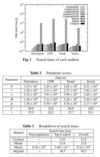
nodes decreases, the size of the subgraphs becomes smaller and searches can be performed at higher speed. This is be- cause if there are fewer query nodes, the set of nodes in the subgraph given by Eq. (27) becomes smaller. The relation- ship between the number of query nodes and the search time is shown in Sect. 5.
We introduce the following lemma to illustrate the properties of subgraphs.
Lemma 10(Upper/lower bounds of subgraphs): The up- per/lower estimated values of selected nodes at thei-th it- eration can be computed fromViandEi.
Proof As described above, pi[u] is the probability that a random walk of lengthistarting from a query node will end up at nodeu. So if a node is situated more thanihops away from a query node, its random walk probability at thei-th it- eration must be 0. As a result, we can obtain the upper/lower estimated values from node setHiand the set of edges that are incident toHi. From Eqs. (2), (3) and (11), it is clear that, if the set of nodesSi is unreachable from a node, then the node’s random walk probability will not affect the estimated upper or lower bounds of any node inSi. This indicates that it is possible to compute the upper and lower bounds of nodes included in setSi from node setRi and the set of edges between nodes inRi. As a result, we need only node setVi=Hi∩Riand edge setEi={(u, v)∈E:u∈Vi, v∈Vi} to obtain the upper/lower estimated values of the selected
nodes in thei-th iteration.
This proof implies that we can use subgraphs to com- pute random walk probabilities and estimate upper/lower bounds for selected nodes. Subgraphs can be used to effi- ciently compute upper and lower bounds as follows:
Definition 7(Computing probabilities by subgraphs): If Ci[u] is the set of nodes that are incident to nodeuin the subgraphGi, then we can compute the random walk proba- bilitypi[u] of nodeuat thei-th iteration as follows:
pi[u]=
q[u] (i=0)
v∈Ci[u]W[u, v]pi−1[v] (i0) (29) The above equation can be obtained by replacingC[u]
withCi[u] in Eq. (2). To find the top-knodes at high speed, we use the above formula to calculate the probabilities of random walks from the subgraph. We use Definitions 2 and 1 to obtain the upper and lower bounds of nodes respec- tively. The naive approach processes the whole graph to calculate these bounds, but by using subgraphs we are able to compute these estimated values more efficiently.
However, it can be computationally expensive to con- struct these subgraphs if the approach of Definition 6 is ap- plied directly, because all the nodes in the graph are used, and this can make it impossible to construct subgraphs effi- ciently. We therefore introduce an incremental approach to obtaining subgraphs that utilizes a set of nodes,hi, and a set of edges,ei, in iterative computations. Here,hi is defined as the set of nodes that areihops away from a query node.
Therefore,h0 = H0 = Q, andHi = i
j=0hj = Hi−1 +hi.
Also,eiis the set of edges that link node setshiandHi−1. That is, sinceHi=Hi−1+hi, we haveei ={(u, v)∈E:u∈ hi, v ∈Hi−1 oru ∈Hi−1, v∈hior u∈ hi, v∈hi}. Note that hiandeican be obtained from a single breadth-first search rooted on the query nodes; whereby hi and ei can be ex- tracted with low computation cost in timeO(N+M). For setshiandei, we have the following lemma:
Lemma 11(Subgraph inclusion): If the sets of nodes and edges are denoted by Vi = Vi−1+hi and Ei = Ei−1+ei
respectively, then ifi0, we haveVi⊆ViandEi⊆Ei. Proof Ifi0, sinceHi=Hi−1+hiandRi⊆Ri−1, we have the following equation from Eq. (27):
Vi=(Hi−1+hi)∩Ri⊆(Hi−1+hi)∩Ri−1 (30) Therefore, we have
Vi⊆Hi−1∩Ri−1+hi∩Ri−1⊆Vi−1+hi=Vi (31) Ifi0, then from Eq. (28),Vi⊆Vi−1+hi, and so
Ei⊆ {(u, v)∈E:u∈(Vi−1+hi), v∈(Vi−1+hi)} (32) Therefore, sinceVi−1=Hi−1∩Ri−1 ⊆Hi−1:
Ei⊆{(u, v)∈E:u∈Vi−1, v∈Vi−1}+
{(u, v)∈E:u∈Hi−1, v∈hi
oru∈hi, v∈Hi−1oru∈hi, v∈hi}
(33)
As a result,Ei⊆Ei−1+ei=Eiholds.
Based on Lemma 11, we can incrementally construct subgraphs while iterating. For graph Gi given by Gi = {Vi,Ei}, we haveVi=Vi−1+hiandEi =Ei−1+ei, whereby graphGi can be constructed incrementally. That is,Gi can be obtained by adding to graphGi−1 all the nodes that are a hop distance ofi from the query nodes, and their corre- sponding edges. Since (1)Gi ⊆Gi holds according to the above lemma, and (2) setshiandeiinclude nodes and edges that are not included in paths to the setSiof selected nodes, we can compute subgraphGi by performing a breadth-first search to determine the paths toSiin graphGi.
Algorithm 1 shows our incremental approach for sub- graph construction. Ifi = 0, the algorithm initializes the node and edge sets to V0 = Q and E0 = {(u, v) ∈ E : Algorithm 1Subgraph construction
Input: Gi−1, subgraph of previous iteration;hi, set of nodes;ei, set of edges;Si, set of selected nodes
Output: Gi, subgraph in thei-th iteration 1:ifi=0then
2: V0:=Q;
3: E0:={(u, v)∈E:u∈Q, v∈Q};
4:else
5: Vi:=Vi−1+hi; 6: Ei:=Ei−1+ei; 7: Gi:={Vi,Ei};
8: compute paths toSiinGi; 9: computeViandEifrom the paths;
10: end if 11: Gi:={Vi,Ei};
12: return Gi;
Algorithm 2Castanet
Input:G, original graph;c, the scaling parameter;k, number of answer nodes;Q, set of query nodes
Output: A, set of answer nodes 1:i:=0;
2:S0:=V;
3:repeat 4: ifi0then 5: i:=i+1;
6: end if
7: computehiandeiby breadth-first search;
8: computeGiby Algorithm 1;
9: foreach nodeu∈Vido
10: computepi[u] fromGiby Eq. (29);
11: end for
12: foreach nodeu∈Sido 13: computesi[u] by Eq. (3);
14: computesi[u] by Eq. (11);
15: end for 16: ifi=0then
17: computeLiby Eq. (19);
18: else
19: if|Li−1|kthen 20: computeLiby Eq. (24);
21: else
22: Li:=Li−1; 23: end if 24: end if 25: if|Li|=kthen
26: computeDiby Eq. (20);
27: else 28: Di:=∅; 29: end if 30: Si+1:=Li\Di; 31:until Si+1=∅ 32: sort nodes ofDi; 33:A:=Di; 34:return A;
u ∈ Q, v ∈ Q}, respectively (lines 2−3). This is because V0 = H0 ∩R0 = Q∩V = Qfrom Eq. (27). Otherwise, it computes graphGi from the graph of the previous itera- tion,Gi−1(lines 5−7). ViandEiare computed fromGiby performing a breadth-first search (lines 8−9). As shown in Algorithm 1, we can incrementally compute subgraphs without using the whole graph.
4.4 Search Algorithm
Algorithm 2 shows our algorithm (Castanet). It first initial- izes the set of selected nodes (line 2), and computes the sub- graph (lines 7−8). For each node included in the subgraph, it computes the node’s random walk probability (lines 9−11), since these random walk probabilities are needed to estimate the upper and lower bounds (Lemma 10). It estimates the bounds of the selected nodes (lines 12−15). Ifi = 0, it computesLifor the answer-likely nodes according to Defi- nition 3 (lines 16−17). Otherwise, it incrementally updates the setLifromLi−1(lines 18−24). From Eq. (4), if|Li|k thenDi = ∅, soDi is only calculated when|Li| = k(lines 25−26). It then updates the selected nodes (line 30). If the set of selected nodes is empty, then the iterations are termi- nated (line 31). The node ranking is obtained by sorting the nodes of setDiaccording to their upper or lower estimated bounds (line 32). Finally,Diis returned as the set of answer nodes (lines 33−34).
In practice, if several nodes have same edge weights
from adjacent nodes, the nodes can have the same similar- ity for the given query. As a result, the number of answer nodes could be more thank. In that case, upper and lower bounds also have the same scores for such the nodes from Definition 1 and 2. Therefore, if several nodes have the same k-th highest lower bound, our approach checks whether the nodes have the same edge weights from adjacent nodes. If so, we determineDialthoughDihas more thanknodes to rank them; otherwise, we computeLiby iteratively updating upper and lower bounds.
As shown in Algorithm 2, our search method does not need any precomputation. In other words, it can perform ad- hoc searches. Also, our algorithm does not need any user- defined internal parameters. Therefore, it offers the user a simple means of performing PPR searches.
4.5 Theoretical Analysis
This section presents a theoretical analysis of the search re- sults and the computation cost of our algorithm. First, we will present a theoretical discussion on the search results.
Theorem 1(Search accuracy): Our proposed method com- putes the top-knodes with exact ranking.
Proof Algorithm 2 performs computations until the set of selected nodes converges to an empty set, whereupon it returns Di as the set of answer nodes. IfSi+1 = ∅, then Li =Difrom Definition 5. SinceLi ⊇AandDi ⊆Afrom Lemmas 5, 6, 7 and 8, we haveLi=Di=AifLi=Diholds.
Therefore we haveDi =AifSi+1=∅holds. SinceDi =A, the ranking of all nodes in set Di is fixed after achieving convergence. Therefore, we can compute the top-knodes
with exact node ranking.
Next, we discuss the time complexity of our approach.
Letlandtbe the average number of selected nodes and the number of iterations in the proposed method, respectively.
Also, letnandmbe the average numbers of nodes and edges in the subgraphs, respectively. Note that the original method requiresO(N+M)T time.
Theorem 2(Computation cost): The proposed method re- quires, on average,O((l+n+m+klogk)t+N+M) time to find the top-knodes.
Proof Our approach first constructs the subgraph, which takesO((n+m)t+N+M) time. This is because (1) nodes and edges are computed by breadth-first search inO((n+m)t) time in the subgraph at each iteration, and (2)hiandeiare obtained, on average, inO(N+M) time. It takes, on aver- age,O((n+m)t) andO(l·t) time to compute the random walk probabilities and estimate the upper/lower bounds from the subgraphs at each iteration, respectively. We compute the sets of answer-likely nodesLiinO(l·t), and we obtain rank- determined nodesDiinO(klogk·t) time. This is because, in each iteration, we can compute rank-determined nodes inO(klogk) time by exploiting quicksort. After reaching convergence, the answer nodes are sorted to obtain the node