A Rule-Based Expert System for Automatic Segmentation of Cerebral MRI Images

©Research Institute for Integrated Science, Kanagawa University

■Full-Length Paper■

A Rule-Based Expert System

for Automatic Segmentation of Cerebral MRI Images Shanjun Zhang

^1,3

and Kazuyoshi Yoshino

²

1 Department of of Computer Science, The Faculty of Science, Kanagawa University, 2946, Tsuchiya, Hiratsuka-shi, Japan 259-1293, Japan

2 Department of Welfare Systems Engineering, Kanagawa Institute of Technology, 1030 Simoogino, Atsugi-shi. Kanagawa 243-02, Japan

3 To whom correspondence should be addressed (Kanagawa University).

E-mail: [email protected]

Abstract: The interior boundary of medical image is fuzzy in nature. In this paper, proposed is a novel method to segment and classify the MR image of head by fuzzy clustering and fuzzy reasoning. Traditional fuzzy clustering methods are basically statistical ones in which only intensity affinities of the image are reflected. Considering the characteristics of MR image, we constructed a set of knowledge-based rules to set the fuzzy memberships of the pixels of the image by generally using the intensity similarities, positional relationships among multiple spectra MR images, and the shape features of the brain tissues and the mathematics morphological analogy of the brain tissues. Then a coarse-to-fine reasoning method is used to combine the fuzzy memberships of the pixels of the T1- and T2- channels of the image to segment the cerebral tissues into gray matter, white matter, and CSF. Experimental results showed the efficiency of the method.

Keywords: fuzzy clustering, rule base, MRI, segmentation, morphological filter

Introduction

Segmentation of volumetric image data plays a key role in medical image processing, especially as a preprocessing step for quantitative analysis and volume visualization. Most approaches to image segmentation try to separate segments containing pixels with similar intensity. For ai- ding visualization of medical images, it is requi- red to classify organs and other solid masses into tissue types.

Unfortunately, nonuniform intensity levels may exist in tissues of identical compositions. The intensity inconsistencies caused by the effect of inhomogeneity of medical modalities and biologi- cal variations of tissues form the main obstacles for the segmentation of medical images. To solve the problem, many methods, which can be categorized into classical, statistical, structural and knowledge-based methods, have been pro- posed ^1-6).

Classical methods include the use of standard image processing techniques such as threshold,

and edge and region-based techniques. These methods are usually sensitive to noise and do not result in continuous regions ⁵⁾.

Statistical methods assume the tissue region to follow a priori model such as a finite Gaussian mixture, then the parameters are estimated by expectation-maximization algorithm (EM) to obtain the final segmentation ^8-13). The structural app- roaches take the use of morphological pro-perties of the objects to aid the segmentation ^{14, 15)}. Mor- phological filtering has been introduced by Mather on ⁷⁾ with the inception of morphological opening and closing, can simplify images and remove irrelevant features while preserving their fundamental shape characteristics.

Statistical segmentation methods seldom incor- porate geometry of regions within the image, while structural methods often ignore the distri- bution of intensity values within the image when making judgements about boundary properties and measures of homogeneity within regions.

Knowledge-based methods provided a means to combine the statistical and structural methods.

Focused on different facts of the image objects, different knowledge-based methods have been proposed ^17-21).

In this paper, we proposed another knowledge- based approach focused on the intrinsic fuzzy property of the cerebral magnetic resonance image. In the proposed method, a simplified fuzzy c-means algorithm is applied to pre- segment the

T

₁ weighted and

T

₂ weighted magnetic resonance image. The segmented results are deliberately under-segmented and over- segmented to get a set of clusters with fuzzy memberships. After the defuzzification of the under-segmented results, they are used to generate the brain mask and the extra-cranial mask by the special feature values distribution of the

T

₁ and

T

₂ weighted images. While the over-segmented results are used to separate the three main brain tissues- white matter, gray matter and cerebrospinal fluid (CSF) into non-overlapped cliques. Then the statistical features such as means and variations together with the morphological characters are calculated for the cliques. Finally, sets of knowledge based fuzzy rules are used to progressively specify the relationship between the cliques and the tissue class memberships. During the fuzzy reasoning, the spatial correspondence among the hetero- spectral images and the k-nearest neighborhood voting mechanism provided means for crossreferences.

Background

In many medical images, pathological tissues appear without clear-cut frontiers, such that fuzzy set fit to model uncertainty and inaccuracy attached both to image components and image processing results. Fuzzy c-means (FCM) is an effective method to separate the available data set into subgroups to reflect the substructures in the feature space of the data set. Let

1 2 3

( , , , , )

_n

X = x x x L x

be the set of d-dimensional feature vectors, the memberships

μ

_ijcan be iterative- ly calculated by minimizing an objective function of the type

2

1 1 1

( , ) ( )

1

c N c

p

p ij i k

i j k

f U V u x v

p

= = =

= −

≤ ≤ ∞

∑∑∑

₍₁₎

2

1 2 1

( ) , 1 ( )

N kj j

k N

j

kj j

u x

v k c

= u

=

=

∑

≤ ≤

∑

⁽²⁾

Where

V = ( , , , ) v v

_{1 2}

L v

_c is a c-tuple of prototypes,

U = { } μ

_ij is the fuzzy partition matrix, and

μ

_j⁼

( μ μ

1_j

,

2_j

, , L μ

_cj

)

denoting the grade of membership of feature point

x

_j.

Usually, the clusters obtained by FCM do not exactly correspond to the tissues to be labeled.

One reason of this is because that it is not known a priori the exact number of the distinct substructures in the image, the other reason comes from the inhomogeneity of the feature values of MR image, such that the pixels of the same tissues may be assigned to different clusters, and in the same cluster, pixels may belong to different tissues. Let

ω

_jbe tissue membership vector of pixel

x

_jas

1 2

( , , , )

j j j Lj

ω = ω ω L ω

⁽³⁾

Where

ω

_ij

∈ [0,1]

^,

i = (1, 2, L L )

and L be the number of tissues. The aim of the rest paper is to provide a novel method to correspond the memberships between

ω

_j^and

μ

j^.

Feature population distribution

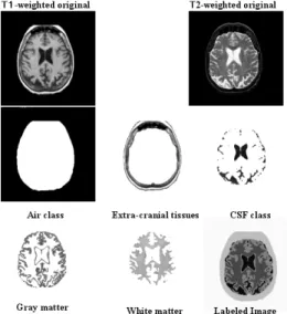
The cross-sectional slices of the MR image consist of three feature images:

T

₁-weighted (

T

₁),

T

₂- weighted (

T

₂), and proton density (PD). The feature values of the images depend on the repetition time (TR) and the echo time (TE) used in scanning.Although the absolute feature values of

T

₁,

T

₂, PD change with person, the relative magnitudes distribution will not change greatly for different tissues.

For example, in

T

₁ feature space, air regions exhibit to be with lowest intensities, white matter exhibit to be with high intensities. The intensities of gray matter are generally lower than those of

white matter but higher than those of CSF. The extra-cranial tissues such as bone marrow, subcutaneous fat, skin has intensities scattering in the range from air to white matter in

T

1feature space. At the mean time, the intensities of the tissues distribute in another but definite form in

T

₂ feature space.

Raya¹⁶⁾ analyzed the histogram of the low-level feature of the tissues and then derived the a set of confidence function to reflect the measure of the likelihood for a class of pixels in the image. Since the histogram of different tissues may overlap, and for a particular tissue, the feature values may vary in several distinct ranges, the resultant confidential function exhibit with overlapped range. To solve the problem, Raya used six low-level features derived by the combination of

T

1 and PD feature spaces.

The idea of ¹⁶⁾ and similar ideas in 13-15, 18, 20)

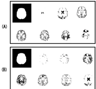
give us motivation to use fuzzy method to describe the certainty a pixel should be assigned to a tissue. We use a simplified fuzzy c-means algorithm to coarsely segment the original image into over-divided clusters. Then we use a set of fuzzy reasoning rules to assign the pixels in each cluster into white matter, gray matter and CSF tissue categories. To reduce the possibility that more than three tissue pixels fall in the same cluster, the number of the clusters is set bigger than the practical for the initial parameter of the

FCM algorithm. IF the number of the clusters be set to be 10, the distribution of the center values of the clusters may follow the spectrum shown in (Fig.1) ²⁰⁾.

Method

Preprocessing

From Fig.1, we can see that it is difficult to separate the extra-cranial tissues merely by the intensities of the feature values. So we take the use of the shape knowledge of the brain to get rid of them.

It is known that brain as a whole is a connected entity, and in

T

₁-weighted image, the intensities of the cranial bone are quite different from those of the air, the image can be approximately be viewed as two parts: air part, and in cranial part;

while in the

T

₂-weighted image, the intensities of the tissues between the cranial bone and the boundary of the brain matters are similar to those of air, and the image can be approximately be viewed as brain-matter part and non-brain- matter part.

By using under-segmented FCM algorithm, we can automatically pick out a cluster as shown in the middle of Fig.2 from the FCM clustering results where the cluster number be set four, and iteration number be set three. Then we can obtain the brain mask and extra-cranial mask through morphological closing processing.

Using the masks, we can separate the bone, skin, fat, and the brain matters from the original Fig. 1. Cluster centers distribution feature of MR

images. (A)

T

₁-Weighted image, (B)

T

₂^-Weighted

image.

Fig. 2. An example of the pre-process. (A) shows the original T₁ -weighted image, a cluster of FCM of T1-weighted image and the outline mask of the head. (B) shows the original

T2-weighted image, a cluster of FCM of _T2-weighted image and the outline mask of the brain.

images. By setting the cluster number eight, the FCM can divide the masked image into six to eight clusters (one or two clusters may be empty when the cluster number be eight), and centers of the clusters may exhibit a distribution as shown in Fig.2. So the pixels in the over-segmented FCM clusters may belong to only one tissue or two adjacent tissues. Next, we will introduce a set of fuzzy rules to separate them by calculating the fuzzy.

Fuzzy rules for tissue membership

In Fig.3, we can see that in the

T

₁ feature space, apart from the extra-cranial regions, the pixels in the lowest two or three clusters may belong to CSF tissues, and those in the highest one or two clusters may belong to white matter, the remain pixels in the two or three clusters in the middle range may belong to gray matter.

Without losing generality, let

μ

_ijdenote the membership of pixel

x

_jto cluster

i

,

v

_idenote the means of the cluster center, where

v

_m

< v

_n^,

form n< ^{, and}

i = (1, 2, , ) L c

. In this subsection we describe a way to transfer the cluster member- ship

μ

_j

= ( μ

_1j

, , L μ

_cj

)

into tissue membership

(

1

, )

j j Lj

ω = ω L ω

. In this paper, c is set eight, and

L

three.

First, the maximum defuzzification method is used to get c clusters from the result of FCM.

Then the statistic characters and the morphological

characters are calculated for each cluster. By statistic characters we mean the average and variation of the cluster. By morphological character we use a ratio

N

_open

N

_orig to represent the cluster's morphological density, where

N

_open is the number of the pixels of the cluster after performing an opening morphological filter on a

3 3× neigh- borhood, and

N

_orig is the number of the pixels of the focused cluster.

Fig.4 shows the defuzzified results of the FCM for

T

₁ and

T

₂- weighted image. Fig.5 shows the distribution of the statistical and morphological features of the corresponded clusters (In the left part, the size of the circle represent the variation of the cluster, and the center of the circle represent the average of the cluster; In the right part the bar represent the morphological density of the cluster). Generally, the value of morpho- logical density of gray matter is small, while those of the white matter or CSF are relatively bigger, and the values change significantly bet- ween the adjacent different tissue clusters.

Combining the vague observed facts from MRI images, we constructed a set of fuzzy rules to assign the memberships of the pixels for the three main brain tissues. In the following rules, four thresholds of

α

₁^,

α

2^,

β

1^,

β

2 are imperatively selected as 0.25, 0.15, 25.0 and 30.0. The parameters may be optimized through a training neural network system in the future.

Fig. 4. Over segmentation results of FCM for a normal image (slice34), (A) is for

T

₁ -weighted image,(B) is for

T

₂-weighted image.

Fig. 3. Cluster centers distribution after mask process. (a) is for - weighted image, (b) is for - weighted image.

membership of the pixels to the three main tissues.¹

T T₂

Rule basees for

T

₁-weighted image

For

T

₁-weighted image, it is easy to say that the pixels in the cluster with lowest average value are a part of CSF tissues and the pixels in the cluster with highest average value are a part of white matters from fig.3. The remained middle clusters are then assigned with CSF and gray matter or gray matter and white matter with fuzzy memberships.

(A)The following rules take CSF as the tissue of the focus-of-attention.

100: if

x

_j belongs to the second lowest cluster then set the membership of

x

_j with

ω

_{csf j,} ^=1.0.

110: if

x

_j belongs to the third lowest cluster then

x

_jwill probably be CSF or gray matter, and the membership of CSF will be set in the range of [0.6,1.0] according to the sub-rules.

111: if the difference of the morphological density to the next cluster (possibly be gray matter) is considerably big, (greater than

α

₁⁾

then set the membership as

ω

_{csf j,} ^=1.0.

112: else if the density difference is relatively great (that is greater than

α

₂, but smaller than

α

1 ^); then assign the membership of

x

_j as

, csf j

ω

^{= 0.9,}

ω

gray j, ^{= 0.1.}

113: else if the difference of the feature value of

x

j and the average value of the known CSF is quite small (less than

β

₁^{); then set}

ω

csf j, ^=0.8.,

, gray j

ω

^=0.2.

114: else if the feature value difference is relatively small (less than

β

₂but greater than

β

1^{); then set}

ω

csf j, ^{= 0.7,}

ω

gray j, = 0.3; else set

, csf j

ω

^{= 0.6,}

ω

gray j, ^=0.4.

(B) The following rules take white matter as the tissue of the focus-of-attention.

200: if

x

_j belongs to the upper most cluster;

then the membership of

x

_j be set

ω

_{white j,} ^{= 1.0.}

210: if

x

_j belongs to the second cluster from the top; then

x

_j will probably be white matter, we refer (Rule 211-213) for further decision.

211: if the difference of the morphological density with the adjacent next cluster is big (greater than

α

1^); then the membership of

x

_j be set

ω

_{white j,} ⁼

1.0.

212: else if the difference is medium (greater than

α

₂but less than

α

₁⁾ then the membership of

x

_j be set

ω

_{white j,} ^{=0.9, and}

ω

gray j, ^=0.1.

213: else if the difference is small, but the morphological density itself is less than 0.5 (it is not clear whether it should be white matter or gray matter); then the membership of

x

_j be set

, white j

ω

^{=0.6, and}

ω

gray j, ^{=0.4; else}

x

j may possibly be white matter, refer(Rule 213a-213c).

213a: if the difference of the feature value of

x

_j

with that of the average of white matter is less than

β

₃ then the membership of

x

_j be set

, white j

ω

^{=0.9, and}

ω

gray j, ^=0.1.

213b: else if the feature value difference is less than

β

₁^; then the membership of

x

_j be set

, white j

ω

^{=0.8, and}

ω

gray j, ^=0.2.

213c: else the membership of

x

_j be set

ω

_{white j,}

=0.7, and

ω

_{gray j,} ^=0.3.

(C) The following rules take gray matter as the focus-of-attention tissue

300: if the difference of the morphological density between the clusters

x

_j belongs to and that of white matter or of CSF is big (greater than

α

1^{); then}

x

j is more likely to be gray matter, and the sub-rules are considered.

301: if the difference of the feature value of

x

_j

Fig.5. Distribution of the statistical and morphological features of the segmented clusters (

T

₁:upper,

T

₂:lower).

with that of the average of white matter or of CSF is greater than

β

₂^; then set the membership of

x

j to be

ω

_{gray j,} ^=1.0.

302: else set the membership of

x

_j to be

, gray j

ω

=0.8, and if the feature value of

x

_j more near to that of the average value of white matter;

then set

ω

_{white j,} =0.2 else set

ω

_{csf j,} ^{= 0.2.}

310: else if the morphological density is not big, but the feature value difference with CSF is bigger than

β

₂^{; then}

ω

gray j, = 0.8, and

ω

_{csf j,} ^{= 0.2.}

320: else if the feature value difference with white matter is bigger than

β

₂^; then set the membership to be

ω

_{gray j,} ^{=0.8, and}

ω

white j, ^=0.2;

else set the membership to be

ω

_{gray j,} ^{=0.6, and}

, white j

ω

^=0.2,

ω

csf j, ^{= 0.2.}

Similar rule-bases are built for

T

₂-weighted feature space, where the lower two or four clusters are considered with high possibility as white matter, and the upper one or two clusters are considered as CSF with high confidence, the remained clusters will be dealt as gray matter candidates.

Combination of the memberships

The fuzzy tissue memberships derived from the fuzzy knowledge rule-base, for

T

₁ and

T

₂ weighted images may remain ambiguities or even be conflict with each other. The ambiguities and conflicting will finally be cleared in a four-levels reasoning process, where the cluster memberships obtained by fuzzy c-means and the tissue memberships assigned by the fuzzy rule base and a k-nearest neighborhood voting mechanism are used.

At the first level, we pick the pixels both with congenial high tissue memberships to generate a representing initial set for the white matter, gray matter, and CSF, respectively. For example, if the memberships for CSF of pixel

x

_j are both greater than 0.8 in

T

₁ and

T

₂ feature space, the pixel will be finally labeled as CSF pixel.We will loosen the conditions to avoid one of the representing sets of the three tissues being empty.

At this stage, for the un-labeled pixels

x

_j, we compare the fuzzy cluster membership

μ

_ij ^of

T

1 and

T

₂ weighted image, if the maximum clusters are both classified to be the same tissues, and the tissue memberships are both greater than 0.7, then the pixel will be labeled the tissue label. After this stage, the means of the feature values are calculated for the labeled tissues of gray matter, white matter and CSF.

In the third combination level, for the remained unmarked pixels, compare the feature value differences of the pixels with average values of the known tissues, if the difference with a certain tissue is smallest for both channels, and the tissue memberships exhibit no conflict with the tissue, then the pixel will be marked with the tissue label.

Finally, the remained unmarked pixels will be labeled by k-nearest neighborhood voting according to the marked results.

Symmetry analysis

After finishing the segmentation of the image, a symmetric measure index is introduced to test the symmetric degree of the brain tissues.

1

| |

1 ( )

symmetric measure

L R α L R

= + ∗ − +

(4)

As it is known, the brain structure is appro- ximately symmetry. Here parameter

α

^{is used}

Fig. 6. The example of the final labeling results after fuzzy reasoning (for slice 34).

to adjust the permissible symmetric range, and L and R represent the numbers of the pixels in the left and right part of the tissue. With different permissible symmetric range, we can vary

α

^to

calculate the symmetric index (degree1) for the left-right part of the whole tissue, and symmetric index (degree2) for the upper left and upper right or the lower left and lower right part of the quadrant of the tissue.

It is desirable to be provided a mechanism to automatically indicate the possible shape corruption of the tissue and thus pick out the possible abnormal images. To calculate the symmetric indexes, it is necessary to divide the brain into four quadrants. Here the mask image of the brain matter and that of the extra-cranial can be used to do so.

Results and Discussion

Experimental results

The proposed rule-based expert system was used to segment a sample of 36 brain scan slices selected from the normal and abnormal image database of

"The Whole Brain Atlas" project²²⁾ of Harvard University. Our system is implemented on a PC Linux machine with CPU of 400 MHz.

For dealing with a slice, it took 44 seconds to assign label, and 4 seconds to calculate symmetry measure index and help indicating diagnosis assistant messages. Fig.6 showed the final labeling results for a normal slice, and Fig.7 showed the final labeling results for an abnormal image.

In the system, we do not distinguish the tumor tissues from the normal brain tissues. Instead of that, we introduced a symmetric measure index to help judging the segmented

region of the tissues of white matter, gray matter, and CSF.

If the symmetry is significantly collapsed, then the tissue is doubted to be with abnormal. Table 1showed the symmetry measure of Fig.6, and Table 2 showed the symmetry measure of Fig.7.

We have tested 36 data slices in the "Whole Brain Atalas" database, where 10 are abnormal slices, and 26 are normal slices. The segmentation results of the normal slices categorized the brain tissues into CSF, gray matter and white matter reasonable, and the symmetry measure indexes of 25 slices are in normal range.

For the abnormal slices, the tumor tissues may be assigned as CSF, and the symmetry measure indexes are less than 0.5 and suggest possible disease in these slices automatically and warn the physician to check the image carefully.

Conclusion

In this paper, we have explained a rule-based expert system, which can automatically segment and label the cerebral MR image and provide assistant message to indicate possible abnormality in the image. Yet the medical physicians should make the final diagnostic decisions. In the system, the image features of the multi-spectral MR intensity distribution, the fuzzy membership of the FCM, and the mor- phological properties of the region are well combined to provide a step-by-step way to achieve consistent tissue labeling.

Experimental results showed the efficiency of the

Fig. 7. The example of the labeling results of an abnormal image.

Table 1. The automatic diagnostic assistant results of example one (normal image of slice 34)

system. The parameters in the system are empirically determined through trial-and-error. Although the selected parameters worked well for most cases, better parameters should be automatically assigned by a training neural network in the future.

References

1) Dawant BM, Zijdenbos P and Margolin RA (1993) Correction of intensity variations in MR images for computer aided tissue classification. IEEE Trans. Med.

Imag. 12: 770-781.

2) Lim KO and Pfefferbaum A (1989) Segmentation OF MR brain images into cerebrospinal fluid spaces, white and gray matter. J. comput. Asisst. Tomogr.

13: 588-593.

3) Brummer ME, Mersereau RM, Eisner RL and Lewine RRJ (1993) Automatic detection of brain contours in MRI data sets. IEEE Trans. Med. Imag. 12: 153-166.

4) Zhang S, Hamabe H and Maeda J (1998) A hybrid approach to segmentation of two channels cerebral MR images. In : Proc. 4th Intern. Conf. Signal Processing. Beijing, pp. 959-962.

5) Harris GJ, Barta PE, Peng LW, Lee S, Brettschneider PD, Shah A, Henderer JD and Schlapfer TE (1994) MR volume segmentaion of gray matter and white matter using manual thresholding dependence on image brightness. Amer. J. Neuroradiaol. 15: 225-230.

6) Bezdek JC, Hall LO and Clarke LP (1993) Review of MR image segmentation techniques using pattern recognition. Med. Phys. 20: 1033-1048.

7) Matheron G (1975) Random Sets and Integral Geometry. Wiley, New York.

8) Cline HE, Lorensen WE, Kikinis R and Jolesz F

(1990) Threedimensional segmentation of MR images of head using probability and connectivity. J. Comput.

Assist. Tomogr. 14: 1037-1045.

9) Liang Z, Jaszczak RJ and Coleman RE (1992) Para- meter estimation of finite mixtures using the EM algorithm and information criteria with application to medical image procesing. IEEE Trans. Nucl. Sci. 39:

1126-1133.

10) Liang Z, MacFall JR and Harrington DP (1994) Parameter estimation and tissue segmentation from multispectral MR images. IEEE Trans. Med. Imag.

13: 339-348.

11) Taxt T and Lundervold A (1994), Multispectral analysis of the brain using magnetic resonance imaging. IEEE Trans. Med. Imag. 13: 470-481.

12) Chang MM, Teklap AM and Sezan MI (1993) Bayesian segmentation of MR images using 3D Gibbsian priors. In : Image Video Processing, SPIE Proc. 1993, Vol.1903. pp. 122-133.

13) Jernigan TL, Press GA and Hesselink JR (1990) Methods for measuring brain morphologic features on magnetic resonance images. Arch. Neurol. 47: 27-32.

14) Brandt ME, Bohan TP, Kramer LA and Flecher JM (1994) Estimation of CSF, white and gray matter volumes in hydrocephalic children using fuzzy clustering of MR images. Computerized Med. Imag.

Graphics. 18: 25-34.

15) Nazif AM and Levine MD (1984) Low level image segmentation: An expert system. IEEE Trans. PAMI.

6: 555-577.

16) Raya SP (1990) Low-level segmentation of 3D magnetic resonance brain images-a rule-based system. IEEE Trans. Med. Imag. 9: 327-337.

17) Stansfield SS (1986) Angy: A rule-based expert system for automatic segmentation of cronary vessels from digital subtracted angiograms. IEEE Trans. PAMI.

8: 188-199.

18) Dhawan AP and Arata L (1991) Knowledge-based 3D analysis from 2D medical images. IEEE Engineering Med. Biol. 10: 30-37.

19) Gerig G Matin J and Kikinis R (1991) Automating segmentation of dual-echo MR head data. In : 12th INt. Conf. Information Processing. in Med. Imag.

20) Li C, Goldgof DB and Hall LO (1993) Knowledge- based classification and tissue labeling of MR images of human brain. IEEE Trans. Med. Imag. 12: 740- 750.

21) Hu ZP, Pun T and Pellegrini D (1990) An expert system for guiding image segmentation. Computer- ized Medical Imaging and Graphics. 14: 13-24.

22) http://www.med.harvard.edu/AANLIB/home.html Table 2. The automatic diagnostic assistant results

of example two (abnormal image)