九州大学学術情報リポジトリ
Kyushu University Institutional Repository
超特異多項式,保型微分方程式および超幾何級数に 関する研究
中屋, 智瑛
https://doi.org/10.15017/1931729
出版情報:Kyushu University, 2017, 博士(数理学), 課程博士 バージョン:
権利関係:
A Study on Supersingular Polynomials, Modular Differential Equations,
and Hypergeometric Series
Tomoaki Nakaya
Graduate School of Mathematics Kyushu University
January 2018
Acknowledgments
Firstly, the author would like to express sincere thanks to his supervisor Professor Masanobu Kaneko for warm encouragement and valuable comments, and for introducing him to the study of the connection between modular forms and supersingular polynomials. He would also like to thank Professor Hiroyuki Tsutsumi and Dr. Yuichi Sakai, who introduced him to the study of supersingular polynomials with certain levels. Finally, he would like to thank his parents and brother for their continuous support.
Contents
1 On modular solutions of certain modular differential equation and supersin-
gular polynomials 1
1.1 Modular forms and supersingular polynomials . . . 1
1.2 Construction of the endomorphism . . . 3
1.3 Modular solutions of ϕg,k(f) = 0 and supersingular polynomials . . . 4
2 The number of linear factors of supersingular polynomials 6 2.1 Introduction . . . 6
2.2 Preliminaries . . . 8
2.2.1 Factorization of the Legendre polynomials . . . 8
2.2.2 Supersingular polynomials for Γ0(N) (N = 2,3,4) . . . 8
2.3 Proof of main theorems . . . 11
2.4 Conjectures of higher levels . . . 16
2.4.1 Level 5 and 7 . . . 18
2.4.2 levelN ∈S− {2,3,5,7} . . . 20
2.5 Supersingular polynomials for p= 2,3 . . . 21
3 Notes on a certain modular differential equations 23 3.1 Introduction . . . 23
3.2 Preliminaries . . . 24
3.2.1 Hypergeometric set-up . . . 24
3.2.2 Modular set-up . . . 25
3.3 Algebraic transformation of the hypergeometric series and Kaneko-Zagier equation . . . 28
3.4 Explicit formulas of solutions . . . 29
3.5 Differential relations . . . 33
3.6 Hypergeometric expression of quasimodular forms of weight 2 . . . 35
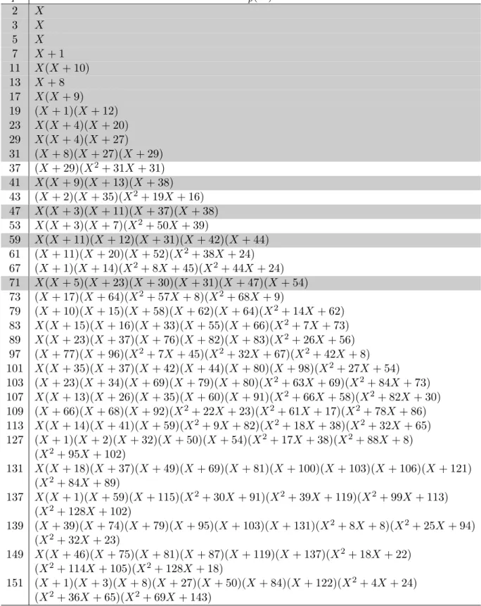
A Factorizations of supersingular polynomials 41
B Orders of sporadic groups 50
Introduction
This thesis consists of three chapters. In Chapter 1, we extend results of Kaneko-Zagier and Baba-Granath on relations of supersingular polynomials and solutions of certain second order modular differential equations. This extended result gives an infinite series of modular differential equations related to supersingular polynomials. In Chapter 2, we focus on the following facts:
the set of prime numbers p such that the supersingular j-invariants in characteristic p are all contained in the prime field is finite. And surprisingly, it is well known that this set of primes coincides with the set of prime divisors of the order of the Monster simple group. In this chapter, we present analogous coincidence of supersingular invariants in level 2 and 3 and the orders of the Baby monster group and the Fischer group. The proof uses a connection between the number of supersingular invariants and class numbers of imaginary quadratic fields. In Chapter 3, we introduce Ochiai’s findings for the solutions of certain modular differential equations studied by Kaneko-Koike and discuss its further implications. Moreover, we use the Ramanujan-Serre differential operator to show that three differential equations related to extremal quasimodular forms, which appeared in the study by Kaneko-Koike, are essentially same. As an application, we simplifies the result on the solutions of certain modular differential equations by Sakai.
Chapter 1
On modular solutions of certain modular differential equation and supersingular polynomials
An elliptic curve E over a field K of characteristic p > 0 is called supersingular if it has no p-torsion over K. This condition depends only on the j-invariant of E, and it is known that there are only finitely many supersingular j-invariants, all being contained in Fp2 . We define the supersingular polynomial ssp(X) as the monic polynomial whose roots are exactly all the supersingular j-invariants:
ssp(X) = ∏
E/Fp E:supersingular
(X−j(E)) .
Because the set of supersingular j-invariants in characteristic p is stable under the conjugation overFp, we have ssp(X)∈Fp[X].
Various lifts of ssp(X) to characteristic 0 are reviewed and studied in Kaneko and Zagier [1].
In particular, they constructed a lift by using a certain differential operator on the space of modular forms. Baba and Granath [2] extended this construction by introducing new differential operators.
In this chapter, we unify and generalize these results, by considering a differential operator arising from a product of Eisenstein series E4, E6, and the discriminant function ∆. With this operator we construct a second-order differential operator which gives rise to an endomorphism of Mk. We write an eigenform of this operator explicitly in terms of hypergeometric series. For k=p−1, we show that the associated polynomial Fe of this eigenform F satisfies
ssp(X) =Xδ(X−1728)εFe(X) mod p, with suitableδ, ε∈ {0,1}.
1.1 Modular forms and supersingular polynomials
For positive even integerk, we denote byMkthe space of holomorphic modular forms of weightk on Γ = PSL2(Z). LetEk(τ) be the Eisenstein series of weight kon Γ defined by
Ek(τ) = 1− 2k Bk
∑∞ n=1
(∑
d|n
dk−1 )
qn (q=e2πiτ),
where τ is a variable in the Poincar´e upper half-plane H and Bk thekth Bernoulli number. For evenk≥4, we haveEk(τ)∈Mk. We also define the discriminant function ∆(τ)∈M12 and the elliptic modular function j(τ) respectively by
∆(τ) = E4(τ)3−E6(τ)2
1728 =q
∏∞ n=1
(1−qn)24=q−24q2+ 252q3−1472q4+· · · and
j(τ) = E4(τ)3
∆(τ) = 1
q + 744 + 196884q+ 21493760q2+· · · . The Gauss hypergeometric series is defined by
2F1(α, β;γ;x) =
∑∞ n=0
(α)n(β)n (γ)n
xn
n! (|x|<1)
where (α)0 = 1 and (α)n=α(α+ 1)· · ·(α+n−1) (n≥1). We note that the series2F1(α, β;γ;x) becomes a polynomial whenα orβ is a negative integer andγ is not a negative integer.
For even k≥4, we can writek uniquely in the form
k= 12m+ 4δ+ 6ε with m∈Z≥0, δ ∈ {0,1,2}, ε∈ {0,1}. (1.1) Under this notation, any modular formf(τ)∈Mk can be written uniquely as
f(τ) =E4(τ)δE6(τ)ε∆(τ)mfe( j(τ))
, (1.2)
where feis a polynomial of degree less than or equal to m. We call fethe associated polynomial of f.
The following representation of ssp(X) is essentially due to Deuring [3]. To be more precise, he proved that the polynomialHp−1(X) of [1, Proposition 5] is equal tossp(X).
Lemma 1. Let p ≥ 5 be a prime number and write p−1 in the form 12m+ 4δ+ 6ε (m ∈ Z≥0, δ∈ {0,1,2}, ε∈ {0,1}). Then
ssp(X) =Xm+δ(X−1728)ε2F1
(
−m, 5
12− 2δ−3ε
6 ; 1;1728 X
)
mod p. (1.3) Proof. We define the monic polynomial Unε(X) of degree n≥0 by
Xn2F1( 1
12,125 ; 1;1728X )
=Un0(X) +O(1
X
), Xn−1(X−1728)2F1
( 7
12,1112; 1;1728X )
=Un1(X) +O(1
X
).
By [1, Proposition 5], we have ssp(X) = Um+δ+εε (X) modp. The first two parameters of the hypergeometric series in (2.1) reduce modulo pto
(
−m, 5
12 −2δ−3ε 6
)
≡
(121,125) (modp) ifp≡1 (mod 12), (125,121) (modp) ifp≡5 (mod 12), (127,1112) (modp) ifp≡7 (mod 12), (1112,127) (modp) ifp≡11 (mod 12).
Since 2F1(a, b;c;x) =2F1(b, a;c;x), we see thatUm+δ+εε (X) is congruent to the left-hand side of (2.1) modulo p.
1.2 Construction of the endomorphism
In this section, we construct an endomorphism ϕg,k of Mk. Let r, s, t be integers, not all zero, and k be an even integer greater than or equal to 4. Then, for the meromorphic modular form g(τ) =E4(τ)rE6(τ)s∆(τ)t̸≡0 of weightu:= 4r+ 6s+ 12tandf ∈Mk, we define the differential operator∂g by
∂g(f)(τ) =∂g,k(f)(τ) =f′(τ)−k u
g′(τ) g(τ)f(τ)
(
′= 1 2πi
d
dτ =q d dq
) ,
and form∈Z≥0, δ ∈ {0,1,2} andε∈ {0,1}withk= 12m+ 4δ+ 6ε, define the operatorϕg,kby ϕg,k(f) = 1
E4
{
(∂g,k+2◦∂g,k)(f)−t2k(k+ 2) u2 E4f
−432
u2 (sk−uε)(sk−uε+ 4(r+ 2s+ 3t))E4∆
E62 f (1.4)
+192
u2 (rk−uδ)(
rk−uδ+ 6(r+s+ 2t))∆ E42f
} .
Note that the function g(τ) is not always a holomorphic modular form. Except for the case of (r, s, t) = (0,0,1), the image off ∈Mk under∂g,k is not holomorphic in general.
Theorem 1. The differential operator ϕg,k is an endomorphism of Mk. To prove the theorem, we need two lemmas.
Lemma 2. The operator∂g is written as
∂g(f) = 4r
u ∂E4(f) +6s
u ∂E6(f) +12t
u ∂∆(f) =∂∆(f) + k 6u
( 2rE6
E4 + 3sE42 E6
)
f. (1.5) Proof. This is easily computed by using the well-known relation (due to Ramanujan)
E2′ = E22−E4
12 , E4′ = E2E4−E6
3 , E6′ = E2E6−E42
2 . (1.6)
Lemma 3. Putv= (sk−uε)/2 andw= (rk−ua)/3. Then
u ∂g,k(E4aE6ε∆c) =vE4a+2E6ε−1∆c+wE4a−1E6ε+1∆c,
u2(∂g,k+2◦∂g,k)(E4aE6ε∆c) = 1728v(v+ 2(r+ 2s+ 3t))Ea+14 E6ε−2∆c+1
+ (v+w)(v+w−2t)E4a+1Eε6∆c (1.7)
−1728w(w+ 2(r+s+ 2t))E4a−2E6ε∆c+1. Proof. One can easily see that the operator ∂∆satisfies the Leibniz rule:
∂∆,k+l(F G) =∂∆,k(F)G+F ∂∆,l(G)
for F ∈ Mk and G∈ Ml. Hence we can prove the lemma by direct calculation using (1.5) and the following relations:
∂∆(E4) =−1
3E6, ∂∆(E6) =−1
2E42, ∂∆(∆) = 0, E43−E26 = 1728∆.
Proof of Theorem 1 For even k ≥ 4, write k in the form k = 12m+ 4δ+ 6ε as before and assume the numbersa, csatisfya≡δ mod 3 (0≤a≤3m+δ),0≤c≤m, andk= 4a+6ε+12c, so that the forms E4aE6ε∆cconstitute basis elements of Mk. We now compute ϕg,k(E4aE6ε∆c).
Since (v+w)(v+w−2t) = t2k(k+ 2)−2t(k+ 1)uc+u2c2, we can obtain from (1.7) the following equation:
u2(∂g,k+2◦∂g,k)(E4aE6ε∆c)−t2k(k+ 2)E4·E4aE6ε∆c
= 1728v(v+ 2(r+ 2s+ 3t))Ea+14 E6ε−2∆c+1+u2c{c−2t(k+ 1)/u}E4a+1E6ε∆c
−1728w(w+ 2(r+s+ 2t))E4a−2E6ε∆c+1.
Furthermore, by using 1728v(v+ 2(r+ 2s+ 3t)) = 432(sk−uε)(sk−uε+ 4(r+ 2s+ 3t)), we have u2(∂g,k+2◦∂g,k)(E4aE6ε∆c)−t2k(k+ 2)E4·E4aE6ε∆c
−432(sk−uε)(sk−uε+ 4(r+ 2s+ 3t))E4∆
E62 Ea4E6ε∆c
=u2c {
c−2t(k+ 1) u
}
E4a+1E6ε∆c−1728w(w+ 2(r+s+ 2t))E4a−2E6ε∆c+1.
We defineλ(x) = 192u2 (rk−ux)(rk−ux+ 6(r+s+ 2t)), then 1728w(w+ 2(r+s+ 2t)) =u2λ(a).
Adding u2λ(δ)E4a−2E6ε∆c+1 to both sides of the above equation and dividing them by u2E4, we get
ϕg,k(E4aE6ε∆c) = 1 E4
{
(∂g,k+2◦∂g,k)(E4aE6ε∆c)−t2k(k+ 2)
u2 E4·E4aE6ε∆c
−432
u2 (sk−uε)(sk−uε+ 4(r+ 2s+ 3t))E4∆
E62 E4aE6ε∆c +48
u2(rk−uδ)(rk−uδ+ 6(r+s+ 2t))∆
E42E4aE6ε∆c }
=c {
c−2t(k+ 1) u
}
E4aE6ε∆c−(λ(a)−λ(δ))E4a−3E6ε∆c+1. (1.8) The right-hand side is an element of Mk if a ≥ 3. If a < 3, we have a = δ (because a ≡ δ (mod 3)) and the coefficientλ(a)−λ(δ) ofE4a−3E6ε∆c+1 vanishes, hence the right-hand side is in Mk. Thusϕg,k is an endomorphism of Mk.
1.3 Modular solutions of ϕ
g,k(f ) = 0 and supersingular polynomi- als
Throughout this section, we assume 2t(k + 1) ̸= cu(1 ≤ c ≤ m) for given r, s, t and k = 12m+ 4δ+ 6ε. By equation (1.8), we see that the matrix representation of ϕg,k in the ordered base{E43m+δE6ε, . . . , E4δE6ε∆m}is triangular matrix and obtain the eigenvaluesc(c−2t(k+1)u ), 0≤ c≤mofϕg,kas diagonal elements. Hence, under the assumption, all eigenvalues of endomorphism ϕg,k are different.
Theorem 2. (i) The following modular form Fg,k(τ) = 1 +O(q) is the unique eigenvector of ϕg,k with eigenvalue 0:
Fg,k(τ) =E4(τ)3m+δE6(τ)ε×
2F1
(
−m, 5
12 +(2r−3s−6t)(k+ 1)
6u −2δ−3ε
6 ; 1−2t(k+ 1) u ;1728
j(τ) )
. (1.9)
(ii) Let k=p−1 wherep ≥5 is prime and assume that u ̸≡0 (modp). Then the associated polynomialFeg,p−1(X) ofFg,p−1(τ) hasp-integral coefficients and
ssp(X) =Xδ(X−1728)εFeg,p−1(X) mod p.
Proof. (i) By using (1.5) and (1.6) to expand the differential equationϕg,k(f) = 0, we obtain f′′(τ) +A(τ)f′(τ) +B(τ)f(τ) = 0, (1.10) A(τ) =−k+ 1
6 E2+k+ 1 3u
( 3sE42
E6
+ 2rE6 E4
) , B(τ) = k(k+ 1)
12 E2′ −k(k+ 1)
36u ·9sE4′E42+ 4rE6′E6
E4E6
+E43−E62 E42E62
{sε(k+ 1)
2u E43−2rδ(k+ 1)−uδ(δ−1)
9u E62
} .
This is a special case of modular differential equations with regular singularities at elliptic points for SL2(Z) treated in [4]. More explicitly, the differential equation (1.10) is expressed as follows using the symbol in [4, Theorem B]:
Dk
(s(k+ 1)
u , 2r(k+ 1)
3u , sε(k+ 1)
2u , 2rδ(k+ 1)−uδ(δ−1) 9u
) .
Applying [4, Theorem C] to this parameters, we get the hypergeometric representation of Fg,k(τ). We note that the exponent of E6(τ) is a solution of the following quadratic equation:
x2−
(2s(k+ 1) u + 1
)
x+2sε(k+ 1) u = 0.
Since ε∈ {0,1}, we have ε(ε−1) = 0 and thus the left hand side of the above equation factor into (x−ε)(x−2s(k+ 1)/u+ε−1). As pointed out in [4, Remark 4], we can choose εas exponent ofE6(τ).
(ii) For k = p−1, by (1.2) and the hypergeometric formula (1.9), the associated polynomial Feg,p−1(X) ofFg,p−1(τ) is as follows:
Feg,p−1(X) =Xm2F1 (
−m, 5
12 +(2r−3s−6t)p
6u −2δ−3ε
6 ; 1−2tp u ;1728
X )
≡Xm2F1 (
−m, 5
12 −2δ−3ε
6 ; 1;1728 X
)
mod p.
Hence Xδ(X−1728)εFeg,p−1(X) is congruent tossp(X) modulo pby Lemma 1.
Remark 1. The case of (r, s, t) = (0,0,1) was studied in the paper [1] by Kaneko and Zagier.
The corresponding operator
∂∆,k(f)(τ) =f′(τ)− k
12E2(τ)f(τ) :Mk→Mk+2 (1.11) is called the Ramanujan-Serre derivative. We note that the logarithmic derivative of ∆(τ) is equal to E2(τ). If k ̸≡ 2 (mod 3), the function F∆,k(τ) coincides with Fk(τ) in [1, Section 8.]
up to a constant multiple. Moreover, Baba and Granath studied the cases of (r, s, t) = (1,0,0) and (0,1,0) in [2]. The corresponding operators are given respectively by
∂E4,k(f)(τ) =f′(τ)−k 4
E4′(τ)
E4(τ)f(τ), ∂E6,k(f)(τ) =f′(τ)−k 6
E6′(τ) E6(τ)f(τ).
Hence, the differential equationsϕE4,k(f) = 0 andϕE6,k(f) = 0 coincides with [2, Eq.(5)] and [2, Eq.(8)] respectively. Consequently, the symbols FE4,k(τ) andFE6,k(τ) we use are same as theirs, but the definition of our operator ϕg,k and their operator ϕare slightly different.
Chapter 2
The number of linear factors of supersingular polynomials
2.1 Introduction
For any prime p ≥5, we define the numbers ν, δ, ε ∈ {0,1}, which will be used throughout this chapter, by
ν = 1 2
( 1−
(−2 p
))
, δ = 1 2
( 1−
(−3 p
))
, ε= 1 2
( 1−
(−1 p
)) ,
where (p·) is the Legendre symbol. We recall Lemma 1 in Chapter 1 : Letp≥5 be a prime and m= [p/12]. Then
ssp(X) =Xm+δ(X−1728)ε2F1
(
−m, 5
12− 2δ−3ε
6 ; 1;1728 X
)
mod p. (2.1) For p = 2 and 3, we have ss2(X) = X mod 2 and ss3(X) = X mod 3 (see [3, p.201]). From this expression we easily see that
degssp(X) =m+δ+ε= p−1 12 +1
4 (
1− (−1
p ))
+1 3
( 1−
(−3 p
)) .
The polynomial ssp(X) factors into linear and quadratic polynomials in Fp[X] by the result of Deuring [3] that all supersingular j-invariants lie in Fp2.
Leth(√
−d) denote the class number of the imaginary quadratic fieldQ(√
−d). The following theorem is essentially due to Deuring ([3, §10] and [5, Eq.(9)]), but is expressed in somewhat different form (see also [6, Lemma 2.6]).
Theorem 3. Ifp≥5, the number L(p) of supersingularj-invariants that lie in Fp is L(p) = 1
4 {
2 + (
1− (−1
p )) (
2 + (−2
p ))}
h(√
−p)
=
1 2h(√
−p) ifp≡1 (mod 4), 2h(√
−p) ifp≡3 (mod 8), h(√−p) ifp≡7 (mod 8).
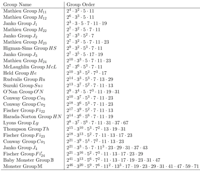
Let M be the monster group. It is the largest sporadic finite simple group and has order
#M= 808017424794512875886459904961710757005754368000000000
= 246·320·59·76·112·133·17·19·23·29·31·41·47·59·71.
In 1975, A. Ogg noticed that the prime divisors p of #M agree with those p such that all characteristic p supersingular j-invariants that lie in Fp (see [7, p.7]). By the definition of the polynomial ssp(X) and the number L(p), Ogg’s observation is paraphrased as the following theorem.
Theorem 4. For a prime numberp,
degssp(X) =L(p) ⇐⇒ p|#M.
This theorem can be proved by using class number estimate, but it does not explain why such a relationship exists.
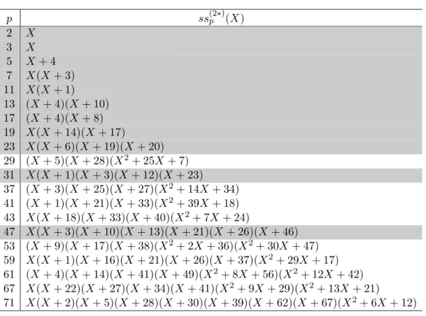
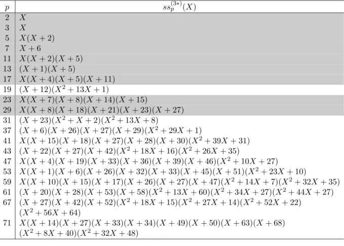
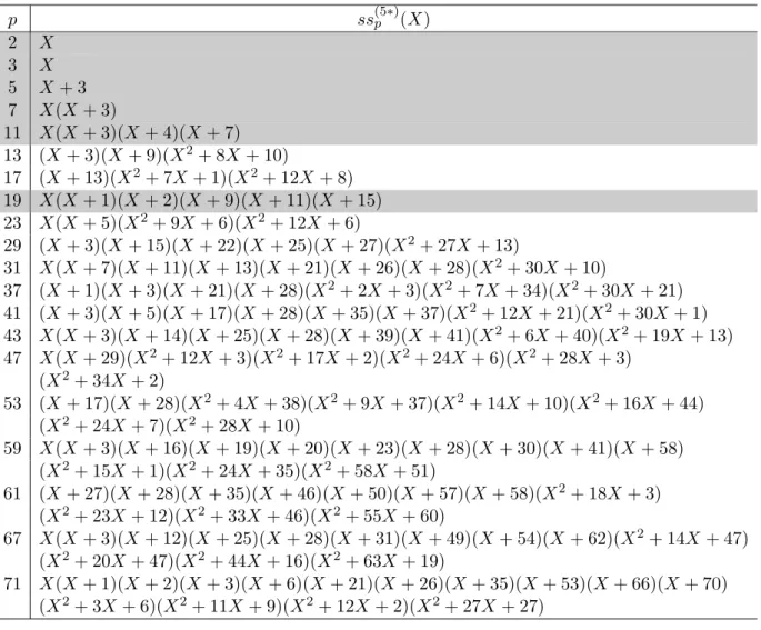
In this chapter, we consider analogues of these theorems in the case of higher levels. The su- persingular polynomialss(Np ∗)(X) for the Fricke group Γ∗0(N) (N = 2,3) was defined by Sakai [8].
It is derived from the invariant differential for Γ∗0(N) (N = 2,3) and has hypergeometric series representation.
Definition 1. For primesp≥5, let m2 = [p/8] andm3= [p/6], and set ss(2p ∗)(X) =Xm2+ε(X−256)ν2F1
(
−m2,3
8 −ε−2ν
4 ; 1;256 X
)
mod p, ss(3p ∗)(X) =Xm3+δ(X−108)δ2F1
(
−m3,1 3+ δ
3; 1;108 X
)
mod p.
For p ∈ {2,3} and N ∈ {2,3}, we have ssp(N∗)(X) = X modp. The degrees of these polynomials are given as follows.
degss(2p∗)(X) =m2+ε+ν= p−1 8 +3
8 (
1− (−1
p ))
+1 4
( 1−
(−2 p
)) , degss(3p∗)(X) =m3+ 2δ = p−1
6 + 2 3
( 1−
(−3 p
)) . We shall prove:
Theorem 5. Ifp≥5 is a prime, then the number of linear factorsL(N∗)(p) ofss(Np ∗)(X) (mod p) is
L(2∗)(p) = 1 8
{ 2 +
( 1−
(−1 p
)) ( 4 +
(−2 p
))}
h(√
−p) +1 4h(√
−2p), L(3∗)(p) = 1
2 (
1− (−3
p ))
L(p) +1 8
{ 2 +
( 1 +
(−1 p
)) ( 2 +
(−2 p
))}
h(√
−3p).
Let Bbe the Baby monster group andF i′24be the largest of Fischer’s groups. The orders of these groups are given by
#B= 4154781481226426191177580544000000
= 241·313·56·72·11·13·17·19·23·31·47,
#F i′24= 1255205709190661721292800
= 221·316·52·73·11·13·17·23·29.
An exact analogue of Theorem 4 for the sporadic groups Band F i′24 holds true.
Theorem 6. For a prime numberp,
degss(2p∗)(X) =L(2∗)(p) ⇐⇒ p|#B, degss(3p∗)(X) =L(3∗)(p) ⇐⇒ p|#F i′24. In Section 2.4, we give some conjectures for higher levels N.
2.2 Preliminaries
2.2.1 Factorization of the Legendre polynomials
Using the theory of elliptic curves, Brillhart and Morton determined the number of linear factors of the following polynomials Wm(x) modp:
Wm(X) :=
∑m r=0
(m r
)2
Xr=2F1(−m,−m; 1;X). (2.2) It is well known that the Hasse invariant for elliptic curves in Legendre form
Eλ :y2 =x(x−1)(x−λ)
isW(p−1)/2(λ) and the elliptic curveEλ is supersingular if and only if W(p−1)/2(λ)≡0 mod p.
Theorem 7 (Brillhart, Morton [9]). Letp≥5 be a prime andN1(p, m) be the number of linear factors of Wm(X) modp. Then
N1 (
p, [p
4 ])
= 1 4
{ 2 +
( 1−
(−1 p
)) ( 4 +
(−2 p
))}
h(√
−p)−ε, N1
( p,
[p 3
])
=δ(2L(p)−1), N1 (
p, [p
2 ])
= 3δ h(√
−p).
We note that the polynomial Wm(X) and the Legendre polynomial Pn(x) := 1
2nn!
dn
dxn(x2−1)n=
(x−1 2
)n∑n r=0
(n r
)2( x+ 1 x−1
)r
satisfy the following relation:
Wm(X) = (1−X)mPm
(1 +X 1−X
)
. (2.3)
Moreover, Morton determined the number of a certain quadratic factors of the Legendre polyno- mials.
Theorem 8 (Morton [10, 11]). Let p≥5 be a prime and B(p, m) be the number of irreducible quadratic factors of the formX2+C of the Legendre polynomial Pm(X) modp. Then
B (
p, [p
4 ])
= 1 4
{ h(√
−2p)−2(ε+ν) }
, B (
p, [p
3 ])
= 1 4
{ aph(√
−3p)−4δ }
, where
ap = 1 2
{ 2 +
( 1 +
(−1 p
)) ( 2 +
(−2 p
))}
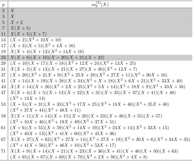
. 2.2.2 Supersingular polynomials for Γ0(N) (N = 2,3,4)
Tsutsumi introduced the supersingular polynomials for congruence subgroups of low levels in [12]
and obtained hypergeometric representations for them. There exist algebraic relations between the elliptic modular invariant j(τ) and modular functionsjN(τ) for Γ0(N) (N = 2,3,4):
(j2(τ) + 192)3−j(τ) (j2(τ)−64)2 = 0,
j3(τ) (j3(τ) + 216)3−j(τ) (j3(τ)−27)3 = 0, (2.4) (j4(τ)2+ 224j4(τ) + 256)3−j(τ)j4(τ) (j4(τ)−16)4 = 0.
We prepare the set
SN :={jN ∈Fp|thej-invariant determined by (2.4) is supersingular}. We then define
ss(N)p (X) = ∏
jN∈SN
(X−jN)∈Fp[X]
for the prime p ≥ 5. Note that we ignore the duplication of elements of the set SN. Because the set SN is stable under the conjugation over Fp, we have ss(Np )(X) ∈ Fp[X]. The following proposition are stated in [12, Proof of Theorem 4] as a congruence relations of ss(Np )(X) and certain polynomial likeUnε(X) appearing in the proof of Lemma 1.
Proposition 1 (Tsutsumi). (i) Let p≥5 be a prime andm= [p/4]. Then ss(2)p (X) =Xm+ε2F1
(
−m,3 4− ε
2; 1;64 X
)
mod p. (2.5)
(ii) Letp≥5 be a prime and m= [p/3]. Then ss(3)p (X) =Xm+δ2F1
(
−m,2 3− δ
3; 1;27 X
)
mod p. (2.6)
(iii) Let p≥5 be a prime and m= [p/2]. Then ss(4)p (X) =Xm2F1
(
−m,−m; 1;16 X
)
mod p. (2.7)
The degrees of these polynomials are given as follows.
degss(2)p (X) = p−1 4 +1
4 (
1− (−1
p ))
, degss(3)p (X) = p−1 3 +1
3 (
1− (−3
p ))
, degss(4)p (X) = p−1
2 .
Proposition 2. If p ≥ 5, the number L(N)(p) (N = 2,3,4) of characteristic p supersingular jN-invariants that lie in Fp is
L(2)(p) =N1 (
p, [p
4 ])
+ε, L(3)(p) =N1 (
p, [p
3 ])
+δ, L(4)(p) =N1 (
p, [p
2 ])
.
Therefore, by Theorems 3 and 7, the numbersL(N)(p) (N = 2,3,4) are constant multiples of the class number h(√−p).
Proof. We only prove the first equality, the other cases being similar. For m= [p/4], Wm(X) =2F1(−m,−m; 1;X) = (1−X)m2F1
(
−m, m+ 1; 1; X X−1
)
and since 34− ε2 ≡m+ 1 (modp), ss(2)p (Y)≡Ym+ε2F1
(
−m,3 4 −ε
2; 1;64 Y
)
≡Yε(Y −64)mWm ( 64
64−Y )
mod p (2.8) Because the number of linear factors is unaffected under the linear fractional transformation of variable, we have L(2)(p) =ε+N1(p,[p/4]) by Theorem 7.
We can regard the polynomial ss(2)p (X) modp as the polynomial part of X[p/4]+ε2F1
(1 4,3
4; 1;64 X
) ,
and hence easy calculation of binomial coefficients gives the following explicit formula ofss(2)p (X).
The case of ss(3)p (X) can be shown similarly.
Theorem 9. For a primep≥5, ss(2)p (X) =
(p−1+2ε)/4∑
n=0
(2n n
)(4n 2n )
X(p−1+2ε)/4−n mod p,
ss(3)p (X) =
(p−1+2δ)/3∑
n=0
(2n n
)(3n n
)
X(p−1+2δ)/3−n modp.
Similarly, we obtain the following theorem concerning the square of supersingular polynomials by applying Clausen’s formula
2F1(α, β;α+β+ 1/2;x)2=3F2(2α,2β, α+β; 2α+ 2β, α+β+ 1/2;x). (2.9) Theorem 10. For a prime p≥5,
ssp(X)2 = (X−1728)ε
(p−1+8δ)/6∑
n=0
(2n n
)(3n n
)(6n 3n )
X(p−1+8δ)/6−n mod p,
ss(2p∗)(X)2 = (X−256)ν
(p−1+6ε)/4∑
n=0
(2n n
)2( 4n 2n )
X(p−1+6ε)/4−n modp,
ss(3p∗)(X)2 =Xδ(X−108)δ
(p−1+2δ)/3∑
n=0
(2n n
)2( 3n
n )
X(p−1+2δ)/3−n mod p.
Here, we would like to point out the similarity between Theorem 10 and the expansions of certain Eisenstein series in terms of 1/j(τ) and similar local parameters described below. By Lemma 1, we have
ssp(X) =Xm+δ(X−1728)ε2F1 (
−m, 5
12 −2δ−3ε
6 ; 1;1728 X
)
mod p
≡
Xm+δ2F1
( 1 12, 5
12; 1;1728 X
)
mod p ifp≡1 (mod 4),
Xm+δ(X−1728)2F1
( 7 12,11
12; 1;1728 X
)
mod p ifp≡3 (mod 4).
We note the following hypergeometric transformation
2F1(α, β;γ;z) = (1−z)γ−α−β2F1(γ −α, γ−β;γ;z) and hence have
2F1 ( 1
12, 5
12; 1;1728 X
)
= (
1−1728 X
)1/2 2F1
( 7 12,11
12; 1;1728 X
) .
It is well known that the Eisenstein series of weight 4 onSL2(Z) has the following hypergeometric representation for sufficiently largeℑ(τ):
E4(τ) =2F1 (1
12, 5
12; 1;1728 j(τ)
)4
∈M4(SL2(Z)).
In [8], it is shown that the Eisenstein series of weight 4 on the Fricke group Γ∗0(N) (N = 2,3) has the following hypergeometric series expression:
(2E2(2τ)−E2(τ))2=2F1
(1 8,3
8; 1; 256 j2∗(τ)
)4
∈M4(Γ∗0(2)), (3E2(3τ)−E2(τ)
2
)2
=2F1 (1
6,1
3; 1; 108 j3∗(τ)
)4
∈M4(Γ∗0(3)).
The calculation of the binomial coefficients using Clausen’s formula (2.9) gives the following:
E4(τ)1/2 =
∑∞ n=0
(2n n
)(3n n
)(6n 3n )
j(τ)−n, 2E2(2τ)−E2(τ) =
∑∞ n=0
(2n n
)2( 4n 2n )
j2∗(τ)−n, 3E2(3τ)−E2(τ)
2 =
∑∞ n=0
(2n n
)2( 3n
n )
j3∗(τ)−n.
These expressions are very similar to the polynomial of Theorem 10. Based on these similarities, we propose conjectural expressions of squares of the supersingular polynomials ss(5p∗)(X) and ss(7p ∗)(X) in Section 2.4.
2.3 Proof of main theorems
In order to prove Theorems 5 and 6, we start with the next proposition on the algebraic relation between the polynomial ss(Np ∗)(X) andss(N)p (X) for N = 2,3.
Proposition 3. (i) Let p≥5 be a prime and m= [p/8]. Then we have (X−64)m+ε+νss(2p∗)
( X2 X−64
)
=Xε(X−128)νss(2)p (X) mod p.
(ii) Letp≥5 be a prime and m= [p/6]. Then we have (X−27)m+2δss(3p ∗)
( X2 X−27
)
=Xδ(X−54)δss(3)p (X) mod p.
Proof. We only prove the case of level 2, the other case being similar. Now m = [p/8] and so p−1 = 4(2m+ν) + 2ε, the polynomial (2.5) is
ss(2)p (X) =X2m+ε+ν2F1 (
−2m−ν,3 4 −ε
2; 1;64 X
)
mod p. (2.10)
Forα=−m−ν/2, β= 3/8−ε/4, we haveα+β+ 1/2≡1 mod p. Based on this, we apply the formula (Kummer’s relation)
2F1 (
2α,2β;α+β+ 1 2;z
)
=2F1 (
α, β;α+β+1
2; 4z(1−z) )
to the right-hand side of (2.10) and get ss(2)p (X) =X2m+ε+ν2F1
(
−m−ν 2,3
8 −ε
4; 1;256(X−64) X2
)
mod p. (2.11)
Ifν = 0, there is nothing to do:
ss(2)p (X) =X2m+ε2F1 (
−m,3 8 −ε
4; 1;256(X−64) X2
)
mod p.
Ifν = 1, we apply Gauss’s relation
2F1(α, β;γ;z) = (1−z)γ−α−β2F1(γ −α, γ−β;γ;z)
to the left-hand side of (2.11). Then the first two parameters of the hypergeometric series of (2.11) reduces modulop to
1−α≡m+3 2 ≡ 3
8 −ε−2
4 , 1−β ≡ 5 8 +ε
4 ≡ −m mod p.
Since the exponent is 1−α−β≡1/2 mod p, (
1−256(X−64) X2
)1/2
= X−128 X . Therefore when ν = 1, we have
ss(2)p (X) =X2m+ε(X−128)2F1
(
−m,5 8+ ε
4; 1;256(X−64) X2
)
mod p.
Summarizing these cases, we finally obtain ss(2)p (X) =X2m+ε(X−128)ν 2F1
(
−m,3
8−ε−2
4 ; 1;256(X−64) X2
)
mod p. (2.12) By multiplying both sides of the above equation by Xε(X−128)ν, we get the assertion:
Xε(X−128)νss(2)p (X)
= (X−64)m+ε+ν
( X2 X−64
)m+ε( X2
X−64 −256 )ν
2F1 (
−m,3
8 −ε−2ν
4 ; 1;256(X−64) X2
)
= (X−64)m+ε+νss(2p∗)
( X2 X−64
)
mod p.
Lemma 4. The roots of W(p−1−2ε)/4(X) over Fp are distinct and all lie in Fp2.
Proof. Firstly, we prove that if λis a root of W(p−1)/2(X), then 1−λis also a root of it. The polynomial Wm(X) = 2F1(−m,−m; 1;X) can be regarded as a polynomial solution of certain hypergeometric differential equation at X= 0 (exponent zero), so this polynomial coincide with the polynomial solution of the same equation atX= 1 (exponent zero) up to a constant multiple.
Since ∑m
r=0
(m
r
)2
=(2m
m
), we have
Wm(X) =2F1(−m,−m; 1;X) = (2m
m )
2F1(−m,−m;−2m; 1−X).
It is easy to see that the congruences( p−1
(p−1)/2
) ≡(−1)(p−1)/2 ̸≡0 (mod p) and−2m≡1 (mod p) hold whenm= (p−1)/2, we have
W(p−1)/2(X)≡(−1)(p−1)/2 W(p−1)/2(1−X) mod p and the first assertion follows.