Power Generation

九州大学学術情報リポジトリ

Kyushu University Institutional Repository

再生可能エネルギー電源を含む電力系統における需 給一致発電計画に関する研究

張, 鵬

https://doi.org/10.15017/1398395

出版情報：Kyushu University, 2013, 博士（学術）, 課程博士 バージョン：

権利関係：Fulltext available.

Generation Scheduling for Supply and Demand Balancing in Power Systems with Renewable

Power Generation

by Peng Zhang

A dissertation submitted in partial fulllment of the requirements for the degree of

Doctor of Philosophy

(Electrical and Electronic Engineering) in Kyushu University

2013

Doctoral Committee:

Professor Junichi Murata, Chair Professor Taketoshi Kawabe Professor Junya Suehiro

⃝ c Peng Zhang 2013

ABSTRACT

The installation of renewable power generation makes a good eort on reducing the emission of greenhouse gas. However, the outputs of some renewable generations are highly aected by nature condition, which contains the uctuation and uncertainties. Therefore, this thesis aims to keep the supply and demand balance in power systems with renewable power generation. For this purpose, three issues are investigated in this thesis: the solar insolation prediction, the error estimation of solar insolation forecasts, and the economically optimal generation scheduling of controllable generators.

First, this thesis improves the wavelet-based solar insolation prediction method which is one of the good prediction methods proposed so far. Given that some variables are well relevant in some time-frequency domains of solar insolation but are weakly relevant in other domains, this thesis only uses the well relevant time-frequency components of a certain input variable instead of its all time-frequency components to predict the value of solar insolation.

The results of a comparison indicate that the proposed method is more accurate than the method which uses the same input variables in all time-frequency domains. Therefore, selecting relevant input variables in dierent time-frequency domains independently is helpful to improve the accuracy of wavelet-based prediction method.

Second, this thesis puts forward the error estimation method, which can extract extra

useful information about the solar insolation from the input variables employed in the solar insolation prediction to complete the forecast results of solar insolation. The errors of solar insolation forecasts are unavoidable, and some of them are extremely big which cause either the large under expectation or large over expectation of PV outputs. However, no relevant researches have focused on estimating the errors of forecasts yet. Therefore, this thesis also focuses on the error estimation of solar insolation forecasts. Given that some big errors concentrate in a certain interval of a variable, this thesis extracts the signicant variables and areas to tell the big errors (positive and negative). The proposed error estimation method can provide the operators with what types of error the forecast is likely to have with high condence using only the input variables employed in solar insolation prediction and the predicted solar insolation. The results of error estimation are useful for operators to identify the extreme situations which cause the large deviation of power.

Finally, this thesis proposes a useful strategy to deal with the uncertainties of forecasts of renewable generation outputs, which can achieve the economically optimal generation schedule with the less total cost compared with the conventional methods, which use the spinning reserves to prevent the possible imbalance incurred by the uncertainties of forecasts.

The optimal generation schedule is necessary considering both the supply-demand balancing and the economy of generation. The conventional methods minimize the operation cost with a constraint to guarantee that the operating generators can readily change their outputs to meet the net load demand variation. High penetration of renewable power generation makes it harder for operating generators to compensate the variation of forecasts. The events of supply-demand imbalance happen more often, and the shortage or excess of electric should be compensated from the outside power systems. Therefore, in this research, the damage caused by possible supply-demand imbalance arising from the large uncertainties of forecasts

of renewable generation outputs are evaluated by penalty which represents the necessarily additional cost to x the imbalance. Due to the random nature of the forecast errors, the penalty is evaluated as an expectation. The optimal generation schedule is obtained by minimizing the summation of expectation of penalty and the operation cost. The proposal is validated by the simulation results.

DEDICATION

To the people who care about me, and look after me.

To my family.

ACKNOWLEDGMENT

It would not have been possible to write this doctoral thesis without the help and support of the kind people around me. I would like to express my deeply gratitude to all of them.

I am extremely grateful to my advisor, Professor Junichi Murata, for his thoughtful guid- ance, unconditional support, great patience, and consistent encouragement during the past three years. I very appreciate the meetings with Professor Murata, where he is always pa- tient of my unclear explanation and immature proposal, and he always provides the scientic discussion and insightful advice. He is my best role model for a scientist and teacher. I also thank the other members of my thesis committee, Professor Taketoshi Kawabe and Professor Junya Suehiro, for their helpful suggestions.

I have also been very fortunate to receive the useful advice from Dr. Hirotaka Takano.

He generously oers many help on my research and life, and he is a nice mentor for me.

I am indebted to China Scholarship Council. Without their nancial support, I cannot nish my doctoral program. I am also thankful to Kyushu University for oering the award of tuition free.

It is a great pleasure to study and research in the System Design Laboratory. I would like to thank Dr. Anan Kaku, Mr. Kaijiang Yu, Ms. Wenjing Cao, and other members in this laboratory for their constructive suggestions, valuable discussions, and normal support.

I want to thank the love of my father Shixiang Zhang, my mother Guimin Guo, and my relatives, who encourage me and support me as always.

LIST OF PUBLICATIONS

P. Zhang, H. Takano, and J. Murata, Daily solar radiation prediction based on wavelet anal- ysis, SICE Annual Conference (SICE), 2011 Proceedings of, pp. 712-717, 13-18 Sept. 2011.

P. Zhang, H. Takano, and J. Murata, et al., Optimal Generation Schedule of Micro-Grids Considering the Uncertainties of Forecasts, Seventeenth International Conference on Intel- ligent System Applications to Power Systems, Tokyo, Japan, 1-4 July 2013.

P. Zhang, H. Takano, and J. Murata, Wavelet-based Daily Solar Insolation Prediction and its Error Estimation, International Conference on Electrical and Electronic Engineering, Xiamen, China, 15-18 July 2013.

P. Zhang, H. Takano, J. Murata, et al., Optimal Generation Schedule in Micro-Grids Consid- ering the Possible Damage by Uncertainties of Forecasts, Research Reports on Information Science and Electrical Engineering of Kyushu University, vol 18, no. 2, pp. 75-83, July 2013.

H. Takano, P. Zhang, J. Murata, et al., A determination method for the optimal operation of controllable generators in a micro grid that copes with unstable outputs of renewable

energy generation, IEEJ Transactions on Power and Energy. (Accepted)

TABLE OF CONTENTS

ABSTRACT ii

DEDICATION ii

ACKNOWLEDGMENT iii

LIST OF PUBLICATIONS vii

LIST OF FIGURES xii

LIST OF TABLES xiv

Chapter I. Introduction 1

1.1 Research background and purpose . . . 1

1.1.1 Research background . . . 1

1.1.2 Research purpose . . . 2

1.2 Key issues for achieving research purpose . . . 3

1.2.1 Issue 1: optimal generation schedule considering the uncertainties of forecasts . . . 6

1.2.2 Issue 2: solar insolation prediction . . . 8

1.2.3 Issue 3: error estimation of solar insolation forecasts . . . 10

1.3 Contributions . . . 11

1.4 Dissertation organization . . . 13

Chapter II. Solar Insolation Prediction 14 2.1 Literature review and feature of proposal . . . 14

2.1.1 Literature review on solar insolation prediction . . . 14

2.1.2 Feature of the proposed method . . . 15

2.2 Wavelet-based method of solar insolation prediction . . . 16

2.2.1 Input variables collection . . . 17

2.2.2 Wavelet analysis and data pretreatment . . . 19

2.2.3 Relevant input variables selection . . . 22

2.2.4 Principal components analysis (PCA) and visualization . . . 25

2.2.5 Regression and combination . . . 27

2.3 Simulation results and discussion . . . 28

2.4 Conclusion . . . 32

Chapter III. Error Estimation of Solar Insolation Forecasts 33 3.1 Necessity and objective of error estimation . . . 33

3.1.1 Necessity of error estimation . . . 33

3.1.2 Objective of error estimation . . . 34

3.2 Research position and key feature . . . 35

3.3 Methods for error estimation . . . 35

3.3.1 Denition of signicant variables and areas . . . 36

3.3.2 Signicant variables and areas extracting . . . 37

3.3.3 Judgment on errors . . . 41

3.4 Simulation results and discussion . . . 43

3.4.1 Case study 1: error estimation of daily solar insolation . . . 43

3.4.2 Case study 2: error estimation of hourly solar insolation . . . 48

3.5 Conclusion . . . 50

Chapter IV. Optimal Generation Schedule Considering the Uncertainties of Forecasts 51 4.1 Literature review and feature of proposal . . . 51

4.1.1 Literature review on generation scheduling with the uncertainties of forecasts . . . 51

4.1.2 Feature of proposal . . . 53

4.2 Formulation . . . 54

4.3 Techniques for optimizing the UC and ELD problems . . . 59

4.3.1 Tabu search . . . 62

4.3.2 Modied equal incremental cost method . . . 63

4.4 Simulation . . . 65

4.4.1 Time elements for generation schedule . . . 65

4.4.2 Simulation conditions . . . 66

4.4.3 Simulation results and discussion . . . 69

4.5 Conclusion . . . 74

Chapter V. Conclusions 77

LIST OF FIGURES

1.1.1 Product scenario for oil and gas liquides [1] . . . 3

1.1.2 The world energy consumption [2] . . . 4

1.1.3 Carbon dioxide emissions from 2003 to 2012 [4] . . . 4

1.1.4 Average annual change in carbon dioxide intensity in the 450 scenario [5] . . 5

1.1.5 Shares of world primary energy [7] . . . 5

1.1.6 The output of PV generation [9] . . . 6

1.2.1 A model of power system with the renewable power generation . . . 7

2.2.1 Procedure of solar insolation prediction . . . 17

2.2.2 Square deviation between the 32 input variables and solar insolation in two dierent domains . . . 23

2.2.3 Relations between the rst principal component and solar insolation in four time-frequency domains . . . 26

2.3.1 Predicted value and real value of solar insolation using the proposed method 30 2.3.2 Predicted value and real value of solar insolation using the same variables in all time-frequency domains . . . 31

3.2.1 The relation of the solar insolation prediction to the proposed error estimation 36 3.3.1 The corresponding signicant area for a certain signicant variable . . . 38

3.4.1 Number of occurrence being a signicant variable of negative big errors in

365 target days for 33 variables . . . 46

3.4.2 Number of occurrence being a signicant variable of positive big errors in 365 target days for 33 variables . . . 46

4.2.1 The conditions when penalty happens . . . 58

4.2.2 Relation of expectation of penalty to the output range of scheduled generators in conventional methods . . . 60

4.2.3 Relation of expectation of penalty to the output range of scheduled generators in proposed method . . . 61

4.4.1 Time elements for generation schedule . . . 66

4.4.2 Data of demand and PV outputs . . . 68

4.4.3 PIS of operation intervals from 13:30 to 14:00 . . . 71

4.4.4 PIS of operation intervals from 13:30 to 14:00 considering the maximum PIS and PIE constraints . . . 73

4.4.5 PIS of operation intervals in a whole day . . . 75

4.4.6 PIS of operation intervals in a whole day considering the maximum PIS and PIE constraints . . . 75

LIST OF TABLES

2.2.1 Input variables used to predict solar insolation on dayn . . . 18

2.3.1 Relevant input variables in eight time-frequency domains . . . 29

2.3.2 Relevant input variables of the method using the same variables in all domains 30 3.4.1 Signicant variables and areas for the rst target day in case study 1 . . . . 44

3.4.2 Statistic results for four kinds of judgments in case study 1 . . . 45

3.4.3 Condence of correct error estimation in case study 1 . . . 45

3.4.4 Common signicant areas of the common signicant variables . . . 47

3.4.5 Statistic results for four kinds of judgments applying common signicant variables in case study 1 . . . 47

3.4.6 Condence of correct error estimation applying common signicant variables in case study 1 . . . 47

3.4.7 Input variables used to predict hourly solar insolation . . . 48

3.4.8 Signicant variables and areas in case study 2 . . . 49

3.4.9 Statistic results for four kinds of judgments in case study 2 . . . 49

3.4.10 Condence of correct error estimation in case study 2 . . . 50

4.4.1 Fuel cost coecient of controllable generators . . . 68

4.4.2 Parameters of controllable generators . . . 69

4.4.3 The cost in the period from 13:30 to 14:00 . . . 72

4.4.4 Comparisons . . . 74

CHAPTER I Introduction

1.1 Research background and purpose

1.1.1 Research background

The fossil fuel energy (oil, coal and gas) takes up the high percentage of energy supply among the current energy resources. However, because of the limited resources and the emission of greenhouse gas, the fossil fuels energy is challenged in the future energy market.

On the one hand, the product of fossil fuel energy is decreasing year by year [1] as shown in Fig. 1.1.1 and the price is growing, because the reserves are limited. However the consump- tion of energy keeps increasing in the future [2] as shown in Fig. 1.1.2. The gap between the consumption and the product of fossil energy is expected to be complemented by other non-fossil energy such as the nuclear energy and the renewable energy. However, concerning about the safety, the anticipated role of nuclear power has been scaled back as countries have reviewed policies in the wake of the 2011 accident at the Fukushima Daiichi nuclear power station [3]. On the other hand, the renewable energy is highly encouraged because it is also environment friendly. The 450 Scenario aims to adopt the measures required to prevent the

average global temperature rising by more than 2 Degree Celsius. However, the emission of greenhouse gas is still growing rapidly in the past ten years as shown in Fig. 1.1.3. In order to achieve the goal of 450 scenario, carbon intensity would have to fall in 2020-2035 at almost four times as fast as in 1990-2008 [5] as shown in Fig. 1.1.4. The renewable energy is the good choice for producing the electricity without emission of greenhouse gas. The share of renewable energy in electricity generation was already around 19% in 2010, with 16% of electricity coming from hydroelectricity and 3% from other renewable generations [6]. In many parts of the world, concerns about security of energy supplies and the environmental consequences of greenhouse gas emissions have spurred government policies that support a projected increase in renewable energy sources [3]. As a result, renewable energy sources are the fastest growing sources of electricity generation [2] and the share of renewable energy among the primary energy keeps increasing in the future [7] as shown in Fig. 1.1.5.

1.1.2 Research purpose

The installation of renewable energy resources makes a good eort on reducing the emis- sion of greenhouse gas. However, the outputs of some renewable generations such as the photovoltaic generations and the wind generations are highly aected by nature condition, which contain the uctuation and uncertainty [8]. Take the photovoltaic (PV) generations as an example of the renewable energy resources. Figure 1.1.6 shows the outputs of PV generations, where the uctuation exists naturally and even some variations are very sig- nicant. Keeping the balance between supply and demand is the basic rule of all power systems [10]. However, when the renewable power generations are connected to the utility grid, the uncertainty of renewable generation outputs makes it harder to balance the supply and demand of the power system [11]. Therefore, the motivation of this dissertation is keep-

Figure 1.1.1: Product scenario for oil and gas liquides [1]

ing the supply and demand balancing in the power systems in the presence of the rapidly increasing renewable power generation.

1.2 Key issues for achieving research purpose

Figure 1.2.1 shows a simple model of power system with the renewable power generation, which consists of the load, controllable generators such as the diesel engine generators and fuel cell, and the renewable power generation such as the PV generations and wind turbines. This thesis focuses on the PV generation among the renewable energy sources. The cost reduction of PV panels and technical progress in power electronic conversion and semiconductor devices make PV systems one of the most promising renewable energy sources [12] [13]. Also,

Figure 1.1.2: The world energy consumption [2]

Figure 1.1.3: Carbon dioxide emissions from 2003 to 2012 [4]

Figure 1.1.4: Average annual change in carbon dioxide intensity in the 450 scenario [5]

Figure 1.1.5: Shares of world primary energy [7]

Figure 1.1.6: The output of PV generation [9]

because of distinctive advantages such as simplicity of allocation, high dependability, low maintenance, and lack of noise, the installation of PV generations by the residents continually increases in these years [14]. Therefore, this thesis takes the power system shown in Fig. 1.2.1 but with only PV generations in the renewable power generation part as the example model of power system because of its popularity. For achieving the research aim, the key issues that we have to deal with are investigated.

1.2.1 Issue 1: optimal generation schedule considering the uncer- tainties of forecasts

In some power system models, the energy storages such as the batteries are included to deal with the uncertainty of PV generation. Actually, the energy storage is eective for the

Figure 1.2.1: A model of power system with the renewable power generation

purpose of power supply and demand mismatch mitigation [15]. However, the installation of batteries requires an extra cost. The cost will be very high due to noncompetitive battery price when a large capacity of battery is introduced [16]. Also, the load control can be also an option to respond to the imbalance of supply and demand [17]. For example, some insensitive loads could be inactive when a signicant shortage of power exists. However, the load control is not consumer friendly. In order to keep the supply and demand balance, the generation schedule is obviously necessary. However, the optimal schedule of controllable generators should not only consider the balance but also the economy of generation. There- fore, this thesis address the economically optimal generation scheduling issue for controllable generators in power systems with renewable power generation to keep the balance of supply and demand, which is the essential issue of this research.

The conventional methods treat the problem as a generation cost minimization prob- lem with a constraint called the spinning reserve constraint in order to guarantee that the operating generators can readily change their output to meet the changeable load demand.

However, high penetration of power generations utilizing the renewable energy sources com- plicates the above problem. In extreme cases that the variations of net demand are especially large, the available generation reserves may be unable to prevent the imbalance. Then, the tail events have been occurring more frequently. The conventional methods cannot prevent the power systems from imbalance all the time, so the power exchange with outside power system becomes more important and necessary. Therefore, we should put forward a new strategy to deal with the uncertainties of forecasts in the power systems with high penetra- tion of renewable power generation. The particular statements on comparison between the conventional methods and proposed methods will be shown in Chapter IV.

1.2.2 Issue 2: solar insolation prediction

Basically, the above mentioned issue is the unit commitment (UC) and economic load dispatch (ELD) problem. The UC and ELD problems are the basic and crucial problems in power systems [18]. The UC problem determines a turn-on and turn-o schedule for a given combination of controllable generating units, thus satisfying a set of dynamic opera- tional constraints. ELD determines the generation outputs of turned-on generating units by minimizing the operation cost while generating the power equal to the load demands [19].

The UC and ELD are signicant research applications in power systems that optimize the total production cost to meet the predicted load demand. However, because of the instal- lation of renewable power generation, some load demand is compensated by the renewable generations. In the power systems with high penetration of renewable power generation, the outputs of renewable generation will make a signicant eect on the net demand. Here, the net load demand, which is expected to be generated by the controllable generators, is the dierence of the load demand and the predicted generation supply from renewable power

generation. Also, the outputs of renewable generation highly rely on the weather conditions which are inconstant normally; therefore the outputs are uctuated and uncertain. There- fore, this thesis should forecast the outputs of renewable power generation before dealing with the UC and ELD problem, which is prior issue of this research.

The outputs of PV generations depend on many factors: the characteristics of PV mod- ules (e.g. the type of PV sell, the total size of PV array), the installation of PV (e.g. the orientation from due south, the latitude of location, the angle from horizontal, anything that shades the panels), and the environmental factors (solar insolation, ambient temperature, wind speed) [20] [21]. The above listed factors are considered as the key factors. Most of the factors normally can be measured and controlled. However, the environmental factors contain the uctuation and uncertainty. Therefore, they should be forecasted. The temper- ature and wind speed are available easily because they are usual parameters of the weather reports. Then, the solar insolation is the only unavailable factor, and also it is considered as the most important factor for predicting the outputs of PV generation. Thus, the pre- diction of solar insolation is necessary for forecasting the outputs of PV generation. The outputs of PV generations can be calculated easily when the necessary factors are available.

Reference [22] provides the simple method for calculating the PV outputs when the solar insolation, the temperature and the characteristics of PV modules are available. Then the issue of prediction of PV outputs is transformed to the solar insolation prediction.

Many methods have been proposed to predict the solar insolation. Most of the current methods only analyzed the problem in time domain, while solar insolation time series contains dierent frequency components. Therefore, some researchers decomposed the sequence of solar insolation into several time-frequency domains by wavelet transform and forecasted them in each domain separately with reasonably good accuracies. But, they use the same

input variables in all time-frequency domains. Some input variables are well relevant for predicting solar insolation in some time-frequency domains but can be weakly relevant in other time-frequency domains. Therefore, we focus on the issue of solar insolation prediction to improve the accuracy of wavelet-based prediction methods. The literature review and the feature of proposed method will be declared in detail in Chapter II.

1.2.3 Issue 3: error estimation of solar insolation forecasts

The investigation of solar insolation forecasts indicates that the forecasted solar insola- tion contains the uncertainty, therefore, the errors of prediction always exist. The errors cause the under expectation or over expectation of the renewable generation outputs. Nor- mally, the generation schedule of controllable generators maintains some generation reserves to deal with these under expectation and over expectation of renewable generation outputs.

However, some errors of the forecasts are extremely large and these big errors of forecasts will cause the large over expectation or large under expectation of renewable generation outputs [23]. With the increasing penetration of renewable power generation, the gap be- tween the actual renewable generation outputs and predicted outputs becomes signicant, as a result of which, the generation schedule based on the predicted renewable generation outputs maybe cannot adapt to the actual net demand at all and the failed operation oc- curs [24]. Moreover, no relevant researches have focused on estimating the errors of forecasts yet. Therefore, this thesis should also focus on the issue of the error estimation of forecasts.

The novelty and feature of error estimation will be concretely declared in Chapter III.

To sum up, in order to keep the balance of supply and demand in power systems with renewable power generation (PV generations), three issues are investigated in this research:

1) the solar insolation prediction; 2) the error estimation of solar insolation forecasts; and 3) the economically optimal generation schedule of controllable generators considering the uncertainties of forecasts.

1.3 Contributions

This thesis aims to the optimal generation scheduling of controllable generators in power systems with renewable power generation. In order to achieve the purpose, three key issues are solved and three contributions are achieved in this research.

First, this thesis proposes an useful strategy to deal with the uncertainties of forecasts of renewable generation outputs, when the UC and ELD problems are investigated. The optimal generation schedule of controllable generators is necessary considering both the supply-demand balancing and the economy of generation. The conventional methods min- imize the operation cost with a constraint to guarantee that the operating generators can readily change their outputs to meet the net load demand variation. High penetration of renewable power generation makes it harder for operating generators to compensate the variation, because their forecasts contain signicant errors. Therefore, the events of supply- demand imbalance happen more often, and the shortage or excess of electricity should be compensated from the outside power systems. In this research, the impact caused by possi- ble supply-demand imbalance arising from the large uncertainties of forecasts of renewable generation outputs are evaluated by penalty which represents the necessarily additional cost to x the imbalance. Due to the random nature of the forecast errors, the penalty is eval- uated as an expectation. The optimal generation schedule is obtained by minimizing the summation of expectation of penalty and the operation cost. The simulation results indicate

that the proposed method can achieve the generation schedule with less total cost than the conventional methods.

Second, this thesis improves the wavelet-based solar insolation prediction method. To improve prediction accuracy of wavelet-based solar prediction method which is one of the good prediction methods proposed so far, relevant input variables to solar insolation are selected in each time-frequency domain respectively instead of using the same input variables in all domains. The comparison result shows that the proposed method is more accurate than the method which uses the same input variables in all time-frequency domains.

Third, this thesis puts forward an error estimation method, which can provide more useful information about the solar insolation with high condence and complete the forecast results of solar insolation without any further input variables but only the variables already employed in solar insolation prediction. The errors of solar insolation forecasts are unavoidable, and some of them are extremely big which will cause either the large under expectation or large over expectation of PV outputs. However, no relevant researches have focused on estimating the errors of forecasts yet. Therefore, this thesis also focuses on the error estimation of solar insolation forecasts. According to the proposed method, we can estimate the errors using only the input variables employed in solar insolation prediction and the predicted solar insolation, and inform the PV/power system operators what kind of error the predicted value of solar insolation is likely to have and how much the condence of the correct estimation is. The results of error estimation are useful for operators to identify the extreme situations which cause the large deviation of power. The case studies validate that the proposed method can extract extra useful information from the input variables employed in the solar insolation prediction.

1.4 Dissertation organization

The organization of this dissertation is as follows. Chapter I mainly presents the back- ground of research, the purpose of research, and the key issues for achieving this research.

In Chapter II, one of the key issues, the solar insolation prediction, is investigated. A wavelet-based method is proposed to forecast the solar insolation. In Chapter III, the issue, error estimation of solar insolation prediction, is solved by the statistics method and two case studies are employed to validate the method. Chapter IV proposes a new strategy to deal with the uncertainties of forecasts in power systems with high penetration of renewable power generation, when UC and ELD problems are investigated (the essential issue of this research). It is validated by the results of a comparison with conventional methods. The conclusions are summarized in Chapter V.

CHAPTER II

Solar Insolation Prediction

Solar insolation prediction is considered as the most important factor in the prediction of PV generator outputs. In this chapter, a wavelet-based method for prediction the solar insolation is proposed. With the proposed method we can predict the total amount of solar insolation of the next day and also we can forecast hourly or half-hourly solar insolation of the next day. Here, this thesis addresses the daily solar insolation prediction as an example.

2.1 Literature review and feature of proposal

2.1.1 Literature review on solar insolation prediction

Many researchers have put forward the solutions to solar insolation prediction. Several models have been developed in order to estimate the global solar radiation data, insolation and daily cleanness index on dierent scales (min, hour, day and monthly), based on analyt- ical, numerical simulation and statistical approaches [25]−[37] For the randomicity of daily values or even hourly values, models in the monthly scale can reect the long-term changing trends better than models in daily scale [38]. In order to achieve this, various empirical

models have also been used to predict monthly mean daily global solar radiation all over the world [39]−[43]. The majority of these models may not be suitable for forecasting purposes because of the large amount of empirically determined parameters, which sometimes results in higher prediction errors [44]. Statistical methods based on Markov chains [45], Boltzmann distribution [46], and Autoregressive Integrated Moving Average [47]− [49] are proven to generate accurate forecasting.

As an alternative to the statistical approach, articial intelligence (AI) techniques have the exibility to account for complicated dependencies that are only partially known, where traditional methods have their limits [50]. AI techniques are becoming more and more popular in the prediction of meteorological data such as solar radiation [51]. A review on articial intelligence techniques applied in the eld of solar radiation estimation can be read in [44], where many methods, such as the articial neural network based methods, fuzzy logic based methods, some hybrid methods (e.g. neuro-fuzzy based methods, neural network and wavelet analysis based methods) and so on, are summarized and evaluated. Many researchers focus on the neural network based forecasting methods [52]− [57], because of its advantages such as its ability to deal with non-linear problems, no statistical assumptions required for the source data and so on [58]. Reference [51] argues that a neural network may forecast daily solar irradiation with accuracy with similar to or even better than conventional methods.

2.1.2 Feature of the proposed method

Most of the above methods only analyzed the problem in time domain, while solar inso- lation time series contains dierent frequency components. For example, it contains yearly changes which are considered as the low frequency components and also contains daily

changes which are the high frequency components compared with yearly changes. Mean- while, dierent input variables that aect the solar insolation contain dierent frequency components too. Therefore, some researchers decomposed the sequence of solar insolation into several time-frequency domains by wavelet transform and forecasted them in each do- main separately with reasonably good accuracies [59] [60]. Their results show that the performance of prediction methods is improved by wavelet analysis. But, they use the same input variables in all time-frequency domains. Some input variables are well relevant for predicting solar insolation in some time-frequency domains but can be weakly relevant in other time-frequency domains. Therefore, the proposed method nds, in each time-frequency domain respectively, the relevant components of relevant input variables and uses them for solar insolation prediction. Moreover, the relation of the input variables to solar insolation can be shown to power system operators easily by the proposed method, which is desired by the power system operators.

2.2 Wavelet-based method of solar insolation prediction

This thesis adopts regression equations to predict the value of solar insolation. The training data are solar insolation and input variables measured up to the target date. The whole procedure for predicting solar insolation is shown in Fig. 2.2.1. The techniques used in the procedure will be explained in this section one by one.

Wavelet Transform

Relevant Variables Selection

Principal Component Analysis

Regression

Combination Input Variables and

Solar Insolation

Figure 2.2.1: Procedure of solar insolation prediction

2.2.1 Input variables collection

In order to predict daily solar insolation, the relevant input variables to solar insolation are required. However, we do not know if a variable is relevant to solar insolation or not, before we evaluate it. Therefore, the prior work is to collect the variables that may be relevant to solar insolation.

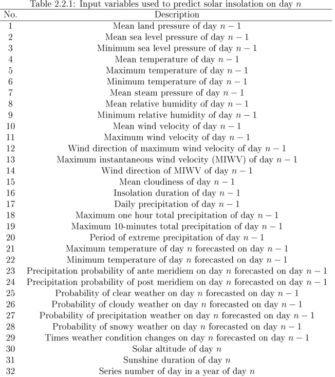
Suppose that n is an index specifying a day. This thesis collects the available variables, which may be relevant to solar insolation, as the input variables. Table 2.2.1 lists the input variables used in this research. These variables are collected because they are used in other researchers' papers or they are easily available weather information. The data vector used to predict solar insolation is dened in Eq. 2.2.1,

Table 2.2.1: Input variables used to predict solar insolation on day n

No. Description

1 Mean land pressure of day n−1

2 Mean sea level pressure of day n−1

3 Minimum sea level pressure of day n−1

4 Mean temperature of dayn−1

5 Maximum temperature of dayn−1

6 Minimum temperature of day n−1

7 Mean steam pressure of day n−1

8 Mean relative humidity of dayn−1

9 Minimum relative humidity of day n−1

10 Mean wind velocity of day n−1

11 Maximum wind velocity of dayn−1

12 Wind direction of maximum wind velocity of dayn−1 13 Maximum instantaneous wind velocity (MIWV) of dayn−1

14 Wind direction of MIWV of day n−1

15 Mean cloudiness of dayn−1

16 Insolation duration of day n−1

17 Daily precipitation of day n−1

18 Maximum one hour total precipitation of day n−1 19 Maximum 10-minutes total precipitation of dayn−1 20 Period of extreme precipitation of day n−1 21 Maximum temperature of day n forecasted on day n−1 22 Minimum temperature of day n forecasted on day n−1

23 Precipitation probability of ante meridiem on day n forecasted on day n−1 24 Precipitation probability of post meridiem on day n forecasted on day n−1 25 Probability of clear weather on day n forecasted on day n−1

26 Probability of cloudy weather on dayn forecasted on day n−1 27 Probability of precipitation weather on day n forecasted on day n−1 28 Probability of snowy weather on day n forecasted on day n−1 29 Times weather condition changes on day n forecasted on day n−1

30 Solar altitude of day n

31 Sunshine duration of dayn

32 Series number of day in a year of day n

f(n) = [f⁰(n), f¹(n), . . . , f^M(n)], (2.2.1)

where f^m(n)(m = 0,1,2, . . . , M) is the original time series of solar insolation (m = 0) and the original time series of the m-th input variable (m = 1,2, . . . , M). M is the number of input variables. N stands for the day whose insolation is to be predicted. f(n) is a set of data on the n-th day dened as the combination of f^m(n)(m= 0,1,2, . . . , M).

{f(1), f(2), . . . , f(N−1)}is the data set used for training the model. When the values of f¹(N), . . . , f^M(N) are obtained, this thesis predicts the target solar insolationf⁰(N) based on the data and the trained model.

2.2.2 Wavelet analysis and data pretreatment

Input variables contain dierent frequency components, and solar insolation has its own specic frequency components. If we can grasp the relations between the solar insolation and the input variables in each of time-frequency domains, we can predict the solar insolation better. Therefore, this thesis pretreats the original daily sequence of each of the input variables and the solar insolation into several sequences which contain dierent frequency components.

Wavelet transform can map the original sequence into dierent time-frequency domains.

The transformed sequences in these time-frequency domains are in time domain, while the frequency components of those sequences reect the dierent parts of frequency components of original sequence [61]. Therefore, we can perform wavelet transform to pretreat original data.

There are two functions in wavelet transform: wavelet bias ψ(n)and scale-function ϕ(n). Discrete wavelet transform (DWT) is dened as Eq. 2.2.2,













W_j,k^d,m =∑

n∈Zf^m(n)ψ_j,k(n) W_j,k^a,m=∑

n∈Zf^m(n)ϕ_j,k(n) j, k = 0,±1,±2, . . .

, (2.2.2)

where W_j,k^d,m and W_j,k^a,m, the results of DWT, are detail coecient and approximation coe- cient of f^m(n) respectively. ψ_j,k(n) is the conjugate ofψj,k(n), and ϕ_j,k(n) is the conjugate of ϕ_j,k(n). ψ_j,k(n)is a series of wavelet bases, andϕ_j,k(n) is a series of scale functions. They are dened as Eq. 2.2.3 and Eq. 2.2.4 respectively,

ψ_j,k(n) =a⁻₀^j/2ψ(a₀^−jn−kb₀), (2.2.3)

ϕ_j,k(n) =a⁻₀^j/2ϕ(a₀^−jn−kb₀), (2.2.4)

where a^j₀ is the scale factor, and kb0a^j₀ is for translation.

The inverse DWT, dened as Eq. 2.2.5, can be used to reconstruct the data sequence, if the functions, {ψ_j,k :j, k ∈Z}, form a tight frame of L²(R). When a₀ = 2 and b₀ = 1, Eq. 2.2.3 and Eq. 2.2.4 become the series of binary wavelets, which form a tight frame of L²(R).

f^m(n) = ∑

kW_J,k^a,mϕ_J,k(n) +∑

kW_J,k^d,mψ_J,k(n)+

∑

kW_J^d,m_−1,kψ_J−1,k(n) +. . .+∑

kW_1,k^d,mψ_1,k(n),

(2.2.5)

where J is the level of wavelet transform. ∑

kW_J,k^a,mϕ_J,k(n) contains the low frequency com- ponents of original time seriesf^m(n). ∑

kW_j,k^d,mψ_j,k(n)includes thej-th level high frequency components of f^m(n) (j = 1,2, . . . , J). [62]

However, the overlap of frequencies happens no matter what kind of wavelet basis is used. Thus, this thesis compares the overlaps among dierent kinds of wavelet basis, and the wavelet basis nameddb20is chosen for its less overlap. Then, this thesis decomposes each sequence of input variables and solar insolation into J + 1 time-frequency domains, shown in Eq. 2.2.6, before selecting the relevant input variables and building proper regression equations,

f^m(n) =∑

uf_u^m(n)

u∈ {(a, J),(d, J),(d, J−1), . . . ,(d,1)},

(2.2.6)

where f_u^m(n) is the low frequency components off^m(n) when u= (a, J), and f_u^m(n) stands for the j-th level high frequency components off^m(n) whenu= (d, j). They are calculated by Eq. 2.2.5. The right side of Eq. 2.2.6 is the nal result of data pretreatment. The original sequence is the summation of the sequences in J+ 1 domains.

2.2.3 Relevant input variables selection

Not all of the input variables are relevant to solar insolation, these irrelevant variables do harm to the regressions. Therefore, we need to select the relevant ones. In wavelet- based methods, the same input variables are always selected for all the time-frequency areas.

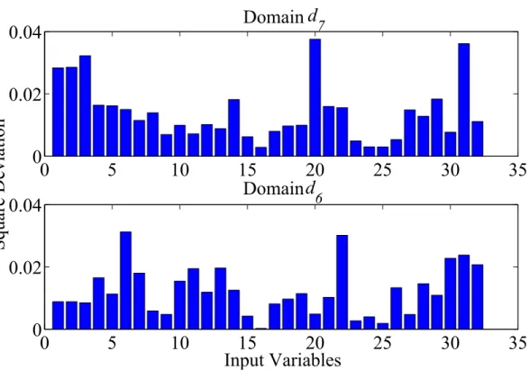
Some time-frequency components of a certain input variable are strongly relevant to the corresponding components of solar insolation, while other time-frequency components of that input variable may be weakly relevant to the corresponding components of solar in- solation. Therefore, the relevant input variables are not necessarily the same in dierent time-frequency domains. Figure 2.2.2 shows, as examples, the square deviations of 32 input variables in two dierent time-frequency domains. The exact denition of square deviation will be given later, and at this stage, it suce to know that a small square deviation indi- cates a relevant input variable. It is clear that the square deviations in dierent domains of a certain input variable are not always small. Take the input variable number twenty as an example. It is signicantly relevant to solar insolation in time-frequency domaind₆, while it is weakly relevant in time-frequency domainsd₇. Therefore we should only choose those well qualied components of the input variable instead of its all components. Thus, well relevant input variables should be selected separately in each time-frequency domain.

The frequency components in each time-frequency domain of input variables are similar to those in the corresponding domain of solar insolation when the dierence between the percentile distribution of spectrum of that variable and solar insolation in the same domain is small. Therefore, this thesis regards the square deviation of percentile distribution of spectrum between solar insolation and input variable in a certain time-frequency domain as the evaluation indicator. First, discrete Fourier transform is performed to f_u^m(n)(n =

0 5 10 15 20 25 30 35 0

0.02 0.04

0 5 10 15 20 25 30 35

0 0.02 0.04

Input Variables

Square Deviation

Domain Domain

d

d

Figure 2.2.2: Square deviation between the 32 input variables and solar insolation in two dierent domains

1,2, . . . , N), so we get the distribution of spectrumF_u^m(z)(z = 1,2, . . . , N). Then, Equa- tion 2.2.7 is employed to achieve the percentage distribution of spectrum.

N(F_u^m(z)) =F_u^m(z)/

∑N z=1

F_u^m(z)×100%, (2.2.7)

where N(F_u^m(z)) are the percentage distribution of spectrum. Finally, we can have the square deviation of percentage distribution of spectrum in time-frequency domain u using the Eq.2.2.8,

D(F_u^m) =

∑Z z=1

(N(F_u^m(z))−N(F_u⁰(z)))², (2.2.8)

where D(F_u^m) is the square deviation of percentage distribution of spectrum between solar insolation and the m-th input variable in the time-frequency domain u. For a certain time- frequency domain, input variables with small square deviation are more relevant to solar insolation in that domain, so they are chosen as the relevant input variables in that time- frequency domain. Then this thesis separately selects the rst S relevant input variables from all 32 input variables in each time-frequency domain. The selected S relevant input variables are represented as in Eq. 2.2.9,

(

f_u^u1(n) f_u^u2(n) . . . f_u^uS(n) )

(2.2.9)

where u_s(s = 1,2, . . . , S) are the serial numbers of the relevant input variables in time-

frequency domain u.

2.2.4 Principal components analysis (PCA) and visualization

The relevant input variables often share the same information, even though this over- lapped information is important to solar insolation prediction. If relevant input variables are highly correlated with each other, it will cause unstable regression results.

PCA is a kind of orthogonal linear transformation which transforms the data into a new coordinate system. The component with the greatest variance after the transformation comes to lie on the rst coordinate; the component with the second greatest variance comes to lie on the second coordinate, and so on [63]. PCA can avoid the cross correlation among the relevant input variables and the unstable regression results. PCA transforms the data in Eq. 2.2.9 to Eq. 2.2.10,

(

g_u^u1(n) g^u_u²(n) . . . g^u_u^T(n) )

, (2.2.10)

whereg^u_u^t(n)(t= 1,2, . . . , T)is the t-th linear combinations of{f_u^us(n)}(s= 1,2, . . . , S) and are the components in new orthogonal coordinate system. u_T is the number of principal components in time-frequency domain u.

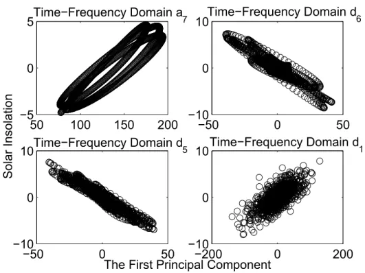
Another reason to perform PCA is to nd the relations between relevant input variables and solar insolation by visualization. Visualization can be performed to nd the relationships between the principle components and solar insolation in each time-frequency domain, if the dimension is reduced to two by PCA. Here, this thesis takes the data of Fukuoka as an example. The cumulative energy content of PCA is set at 99%, therefore only 1% information

50 100 150 200

−5 0 5

−50 0 50

−10 0 10

−50 0 50

−10 0 10

The First Principal Component

Solar Insolation

−200 0 200

−10 0 Time−Frequency Domain d₅ 10

Time−Frequency Domain a₇ Time−Frequency Domain d₆

Time−Frequency Domain d₁

Figure 2.2.3: Relations between the rst principal component and solar insolation in four time-frequency domains

at most can be ignored in the process of PCA. The rst principal component takes up about 60% information of the all relevant input variables. The result of visualization indicates that relations, shown in Fig. 2.2.3, between the rst principle component and solar insolation in all time-frequency domains are linear. So the linear regression equations can be employed.

Note that visualization results can dier and that the relations between the rst principal component and solar insolation may be not linear, if the data are from dierent places in the world.

2.2.5 Regression and combination

A dierent linear regression equation is built in each time-frequency domain, which is based on least square approximation [64]. Then, the prediction of solar insolation is carried out in each time-frequency domain separately, using the principal components of the relevant input variables for the target day N and the linear regression equation of the corresponding time-frequency domain. The linear regression is expressed in Eq. 2.2.11,

fˆ_u⁰(N) =

∑T t=1

(b^u_u^tg^u_u^t(N)) +b⁰_u, (2.2.11)

where fˆ_u⁰(N) is the estimate of solar insolation in the time-frequency domain u for the day N, andb^u_u^t(t = 1,2, . . . , T) are the corresponding regression coecient to the principal component g_u^ut. b⁰_u is the constant coecient. The parameters are estimated based on the data for days 1,2,· · · , N −1,and the prediction is made for the day N.

The nal result of solar insolation prediction for the target day N is the summation of predictions in all time-frequency domains of solar insolation, shown in Eq. 2.2.12.

fˆ⁰(N) = ∑

u

fˆ_u⁰(N), (2.2.12)

where fˆ_u⁰(N) comes form Eq. 2.2.11.

2.3 Simulation results and discussion

The practical example of solar insolation prediction is provided in this section. Also, a comparison is performed between the proposed method and the method using the same variables in all time-frequency domains.

In the proposed method, the input variables are described at the beginning of the Section 2. Data over four years from Jan. 1st, 2006 to Dec. 31st, 2009 at Fukuoka, Japan are used.

(All data are provided by Japan Meteorological Agency). The prediction is performed for each of the days in the last one year in the four years period. For each target day, the past three years (1096 days) data are used for training. As the day proceeds, the newly obtained data are added to the training data set but the oldest ones are eliminated, which keeps the number of training data the same.

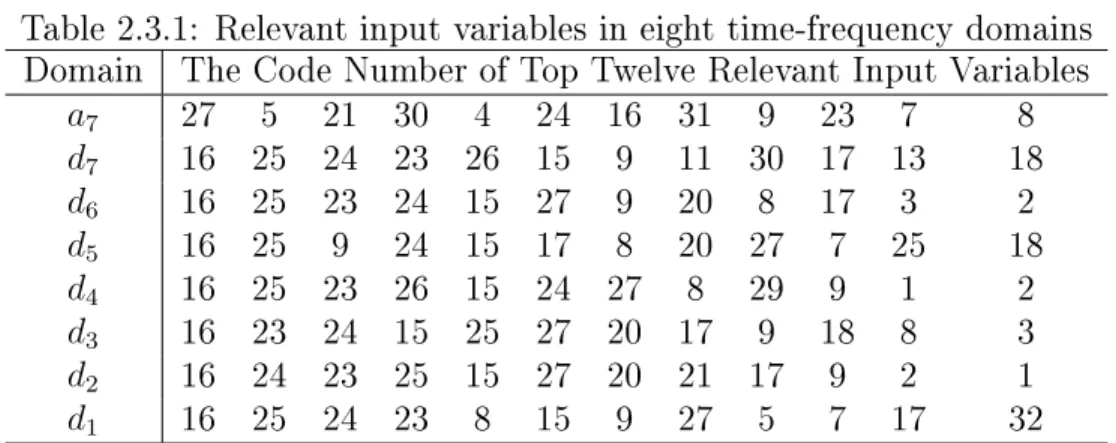
The number of levels of wavelet transform, J, is assigned with seven, so there are eight time-frequency domains totally. Actually, the higher the value of J is, the more accurate the prediction results of low frequency domains are. However, the errors in low frequency domains improves only slightly when the level J is beyond seven. S is set to twelve. The relevant input variables in the eight time-frequency domains are listed in Table 2.3.1. It is clear that the relevant input variables in dierent time-frequency domains are not the same.

Therefore, the relevant input variables should be selected in each time-frequency domain respectively, and also the PCA and regression analysis should be performed respectively.

Then PCA was employed to reduce the dimension. The number of components being selected by PCA diers in dierent time-frequency domains and dierent target days. The range of the number of components is from six to eleven. For one target day, fewer compo- nents are selected in low time-frequency domains than these in high time-frequency domains.

Table 2.3.1: Relevant input variables in eight time-frequency domains Domain The Code Number of Top Twelve Relevant Input Variables

a₇ 27 5 21 30 4 24 16 31 9 23 7 8

d7 16 25 24 23 26 15 9 11 30 17 13 18

d₆ 16 25 23 24 15 27 9 20 8 17 3 2

d₅ 16 25 9 24 15 17 8 20 27 7 25 18

d4 16 25 23 26 15 24 27 8 29 9 1 2

d₃ 16 23 24 15 25 27 20 17 9 18 8 3

d₂ 16 24 23 25 15 27 20 21 17 9 2 1

d1 16 25 24 23 8 15 9 27 5 7 17 32

To understand the relation between the solar insolation and the useful information contained in the relevant input variables, the relations between the solar insolation and the rst prin- cipal component in each time-frequency domain are visualized. The results show that the relations between the rst principle components and solar insolation in every time-frequency domains are linear, which has been already shown in Fig. 2.2.3.

Therefore, the linear regression equation is built in each time-frequency domain respec- tively based on least square approximation using the principal components and solar inso- lation in the corresponding time-frequency domain. The prediction results of the proposed method are shown in Fig. 2.3.1. This gure visualizes the relations between predicted value of solar insolation and the real value of that. The nearer the dot is from the diagonal, the smaller the error is. Basically the dots locate around the diagonal. However, some dots disperse towards the top left corner or the lower right corner of this gure, which are the positive big errors and negative big errors respectively. The root mean square error (RMSE) of the proposed method is 4.27 M J/m².

In order to compare the proposed method with the method using the same variables in all domains, an example of the latter method is implemented. In this method, the relevant input variables are selected based on the square deviation of percentage distribution of spectrum

0 50 100 150 200 250 300 0

50 100 150 200 250 300

Real Value of Solar Insolation (0.1MJ/m²) Predicted Value of Solar Insolation (0.1MJ/m2 )

Figure 2.3.1: Predicted value and real value of solar insolation using the proposed method between the original (not wavelet-transformed) sequences of the solar insolation and the input variables. Therefore this method uses the same relevant input variables in all the time-frequency domains. The selected relevant input variables are listed in Tab. 2.3.2. Then, the wavelet transform and PCA analysis are performed, and a linear regression equation is built in each time-frequency domain. The prediction results are shown in Fig. 2.3.2. The root mean square error is 4.44 M J/m².

Table 2.3.2: Relevant input variables of the method using the same variables in all domains The Code Number of Top Twelve Relevant Input Variables

Solar Insolation 15 14 10 13 12 16 25 11 24 9 23 26

The mean value of actual solar insolation of the 365 target days is about 15M J/m². The

0 50 100 150 200 250 300 0

50 100 150 200 250 300

Real Value of Solar Insolation (0.1MJ/m²) Predicted Value of Solar Insolation (0.1MJ/m2 )

Figure 2.3.2: Predicted value and real value of solar insolation using the same variables in all time-frequency domains

prediction accuracy was improved by 1.3% ((4.44-4.27)/15) of the actual solar insolation by the proposed method. Reference [22] proposes the method to calculate the PV outputs, which indicates that the relation of PV output to solar insolation is direct proportion. Therefore, the proposed method can improve the prediction accuracy of PV outputs by 1.3% of the actual PV outputs. In Japan, the government's plan is to install 53 GW of PV systems by 2030 [65]. Then the expected reduction of prediciton error will be 689 MW, which is similar to the capacity of a normal thermal power plant like the thermal generation unit No. 2 or No.

4 used in Tomato-Atsuma Power Station of Japan [66]. So, this prediction error reduction will have an economical benet equivalent to the starting-up cost of a thermal plant.

2.4 Conclusion

Given that some variables are well relevant in some time-frequency domains of solar in- solation but are weakly relevant in other domains, this thesis only uses the well relevant time-frequency components of a certain input variable instead of its all time-frequency com- ponents to predict the value of solar insolation. Since the dimension of input variables is reduced to less than three by PCA, the relations between the rst principle component and solar insolation in every time-frequency domains are found to be linear based on the data of Fukuoka by visualization. A liner regression equation is built in each time-frequency domain respectively. The results of a comparison indicate that the proposed method is more accu- rate than the method which uses the same input variables in all time-frequency domains.

Therefore, we can conclude that selecting relevant input variables in dierent time-frequency domains independently is helpful to improve the prediction accuracy.

CHAPTER III

Error Estimation of Solar Insolation Forecasts

The solar insolation prediction is necessary for prediction of PV outputs. However no matter what kinds of forecasting methods are applied, there are always some errors in their forecasts and some of them are especially big. Those big errors cause either large under expectation of PV outputs or large over expectation of PV outputs, however no relevant researches have focused on estimating the errors of forecasts yet. Therefore, this chapter focuses on the error estimation of solar insolation forecasts.

3.1 Necessity and objective of error estimation

3.1.1 Necessity of error estimation

The errors are unavoidable no matter what kinds of forecast method are applied. Those errors result from the limitation of forecast method and the lack of necessary information.

We can expect an increase on the average accuracy of forecast by improving the forecast

method, on which many researchers have focused. However, the big errors are unavoidable among the errors of forecasts.

With the increasing penetration of PV generations, the tail events have been occurring more frequently, and magnitudes of imbalance in these events are getting larger [67]. The tail events can be caused by a sudden and signicant power imbalance exceeding reason- able operation reserve capacity [68]. The big errors will cause the large over expectation or under expectation of PV outputs, which increases the probability of imbalance. There- fore, we should focus on these big errors of forecasts in addition to the solar insolation prediction [69] [70]. The types of errors reect the quality of forecast results. One possible application is that if we can judge that the error is likely to be big, then the operators need to make an especially large spinning reserve to compensate the possible large uctuation of PV outputs. On the contrary, if we can judge that the error is not likely to be big, the large spinning reserve is unnecessary.

Therefore, given the two points above, the error estimation is necessary and useful for power system operators.

3.1.2 Objective of error estimation

Actually, those big errors attribute to the lack of information for the solar insolation prediction. In order to avoid the large errors, more information for the solar insolation prediction is necessary. However, such information is normally unavailable or economically inecient. Thus, the best thing that we can do is to extract as more information from the currently used input variables for solar insolation prediction as possible to contribute to the forecasts. Since most of the useful information in the input variables are extracted and used

to predict the value of solar insolation, the remains of the useful information are limited.

The remaining information cannot tell that the error will be a specic value, or whether or not the error will be surely big, because the remaining information is too weak to do so.

Actually, if it were possible, the forecast accuracy would be expected to be increased by improving the forecast method. What we can expect most is that the remaining information is useful to tell the big errors with some certainty. Therefore, this research aims to judge what kind of error the forecast is likely to have and what the condence of correct estimation is without using any further information but only that used in solar insolation prediction.

3.2 Research position and key feature

Figure 3.2.1 shows the relation of the solar insolation prediction to the proposed error estimation. This proposal is based on solar insolation prediction. The benet of this proposal is that the result of solar insolation prediction can be supplemented with additional useful information.

The key feature of the proposed method for error estimation is that the proposed method can extract more useful information on solar insolation without using any extra information but only the available input variables which are used in the solar insolation prediction.

3.3 Methods for error estimation

The error, ∆E, is dened as the value of the predicted solar insolation minus the actual solar insolation. This proposal does not require any extra information but combines the input variables employed in the prediction of solar insolation and the forecasted value of

Input Variables Models for Prediction Predicted Solar Insolation

Input Variables used in Prediction and

Predicted Solar Insolation

Statistics Method Error Estimation Solar Insolation Prediction

Proposed Error Estimation

Categories of Errors and Confidence of Correct Estimation

Figure 3.2.1: The relation of the solar insolation prediction to the proposed error estimation solar insolation together as the input variables for error estimation. This section gives the denition of signicant variable and signicant area which characterize the conditions for big error occurrences, presents the method for nding the signicant variables and their corresponding signicant areas of positive and negative big errors, and proposes a proper way to use them to judge the errors.

3.3.1 Denition of signicant variables and areas

Before giving the denition of signicant variable and area, this thesis denes the cat- egories of errors rst. Suppose that E_pos and E_neg are the thresholds of positive big errors and negative big errors respectively. ∆E is positive big error if ∆E ⩾ E_pos >0, otherwise

∆E is non-positive-big error. ∆E is negative big error if ∆E ⩽E_neg <0, otherwise ∆E is non-negative-big error. ∆E is normal error, if its value isE_neg <∆E < E_pos.

Investigation of big errors (positive or negative) has revealed that they occur with a high probability when the value of a certain input variable is within a certain interval but do not when the value is outside the interval. However, not all of the input variables contain