A time series analysis on the fluctuation of the rate of increase or decrease in the volume of the aquifer of the shallow groundwater in the paddy fields-香川大学学術情報リポジトリ

126 Tech Bull. Fac. Agr, Kagawa Univ

A TIME SERIES ANALYSIS ON T H E FLUCTUATION O F T H E RATE O F

INCREASE OR DECREASE IN T H E VOLUME O F T H E AQUIFER O F

T H E SHALLOW GROUNDWATER IN T H E PADDY FIELDS

Kiyoshi FUKUDA, Katsuhiko I z u ~ s u and Tadao MAEKAWA

1. Introduction

During the period of rise, the water table moves upward from the phreatic low to the phreatic high. Therefore the volume of aquifer increases as time goes on. During the period of decline, the water table moves downward from the phreatic high to the phreatic low, and then the volume of aquifer decreases as time goes on.

When the volume of aquifer is measured for each month, a time se~ies of the volume of aquifer is obtained. From this series, the aquifer's volume of increase during two consecutive months is obtained for the period of rise. And also, the volume of decrease is obtained for the period of decline.

The values of the volumes of increase or decrease show a random variation in their time series. A study of the variations in the time series analysis was made. This paper is the 15th report of "Shallow Groundwater in the Downstream Basin of the Aya River".

2. Theory

The volume of increase or decrease between two consecutive months (dv) can be obtained by Eq. (1).

VMar.- V A ~ I .=dv1 VApr

.-

VMay = dv2

V~an.

-

V~eb

.

= dv 1 1 where

V= The volume of aquifer,

VMar. = T h e volume of V in March, V A ~ ,

.

= T h e volume of V in April,

VFeb. = T h e volume of V in February, and

& = T h e increased (or the decreased) volume o f ' V between two consecutive months. The time series of dv for a year (March to February) can be obtained if the data of

v

for the year is computed by using Eq. (1)" The time series of d v also shows the variation of dv during the year. The degree of variation can be shown by the non-dimensional equation, Eq. (2).

f =- dv v=.Zdv

Vol. 20, No. Z(1969) 127 In order to express mathematically the variation of f for the full year, a harmonic analysis is needed to calculate the FOURIER coefficients for the data of ,f. T o make the analysis, Eqs. (3) and (4) were constructed by applying the FOURIER series.

2 n 2 n 27c

f t =*+al cosK-+a2 cos 2K---+,-,,, .+an cos nK-

2 m m m

2 n 2 n 2 n

+

bl sinK-+ b2 sin 2K-+ ,,,,,,,,,

+

bn sin nK-

m m m ( 3 )

The values of f obtained by Eq. (3) are called the theoretical values of f or

ft

hereafter. In practice, the values of the FOURIER coefficients are computed by using the 12-ordinate scheme with the interval

[O,

2n] representing a year (March to February), m representing 12 months, and fn representing the observed values of f in a month( fo =

f

in March, fl = f in April,

,

f 1 = f in Febr uary).

The values of f fluctuate from the+region to the-region of f. Therefore, in order to see the characteristics of the variation of f , one must estimate the variation of f in the+region only, or in the-region only. As one of the methods of estimating the variation of+ f only, or. -f only, the equation (Eq. (5)) was constructed.

The values of F also mean the cumulative values of f / Z f . In order to express mathematically the curve drawn by the cumulative values of F in the

+

region, Eq.(6) was constructed by applying the GOMPERTZ( 1) curve. In practice, in order to fit the curve to our problem, the

partial total method was used, and then Eq.(7) was constructed.

F t = K a P t ( 6 )

'

I

P " - l \

I O ~ K = ~ 21 Z ~ ~ F -log a ( ~ - ~

where

K = A n asymptote, or limit that the trend values approach as Pt approachesoo. Z1, Z2 and

Z3

=the total for the three parts, respectively, and t = time.

For the cumulative curve of F in the-region, Eq. (8) was constructed by applying the LOGISTIC curve( 1 ), and the values of the constants in the equation were obtained by the selected points method. Eq. (9) was constructed by this method.

128 Tech. Bull Fac.. Agr Kagawa Univ.

where

Fo,

Fl

and

f i

=three selected points (the values of

F

at to, t l and t z , respectively). 3. D a t a

The data used in this paper was obtained from our field investigations ( 2 ) of shallow groundwater

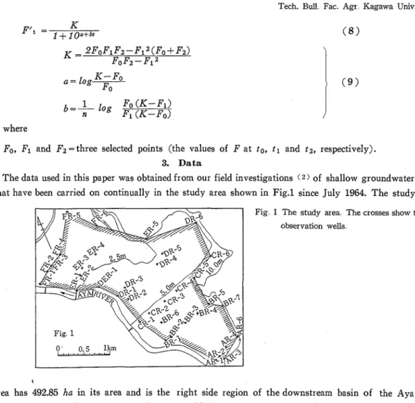
that have been carried on continually in the study area shown in Fig.1 since July 1964. The study

Fig 1 The study area The crosses show the observation wells

1

area has 492.85 ha in its area and is the right side region of the downstream basin of the Aya River, Kagawa Prefecture. TO get the water table data, 36 observation wells(3) ( d l 5m, d=well depth) have been used. They are shown by the crosses in Fig.1.

4. R e s u l t s a n d Discussion

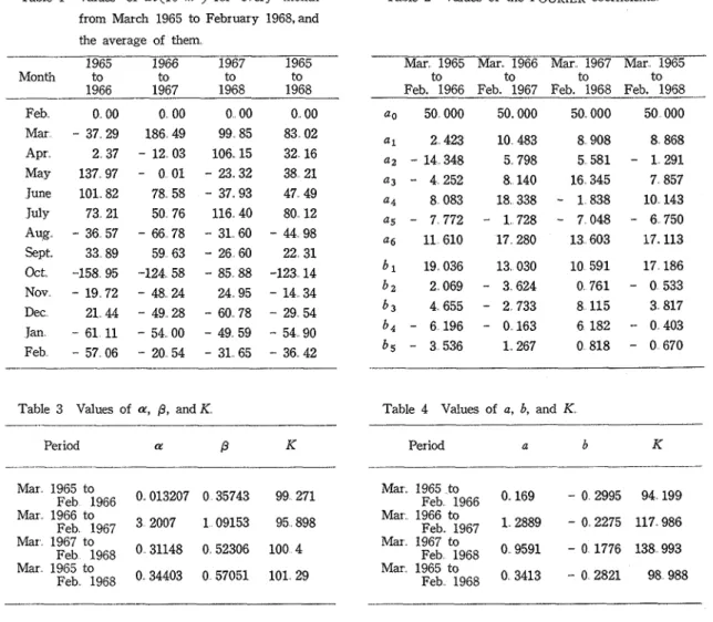
By using this data(4), the time series of dv were obtained by Eq.(l) as listed in Table 1. From Table 1, it is seen that the volume of dv varies from-158.95~ 104m.3 (October 1965) to 186.49

x 104m3(March 1966) throughout the three years (March 1965 to February 1968).

By using Eq.(2), the values of f were obtained and the results of that are shown by the solid circles in Figs. 2 (March 1965 to February 1966), 3 (March 1966 to February 1967), 4 (March 1967 to February 1968) and 5 (the average of the three years). These data of f ' are called the observed data hereafter.

In order to obtain the values of the FOURIER coefficients for our problem, the observed data shown in Figs.2 to 5 was used, and the values of the coefficients were obtained by Eq. (4) as listed in Table 2. By using Eq. (3) with the values of the FOURIER coefficients listed in Table I, the theoretical values of f or ft were obtained as shown by the open circles in Figs. 2 to 5.

These figures tell us the theoretical values (the open circles) are close to the observed ones (the solid circles) throughout the years.

Vol.. 20, No.. 2(1969) 129

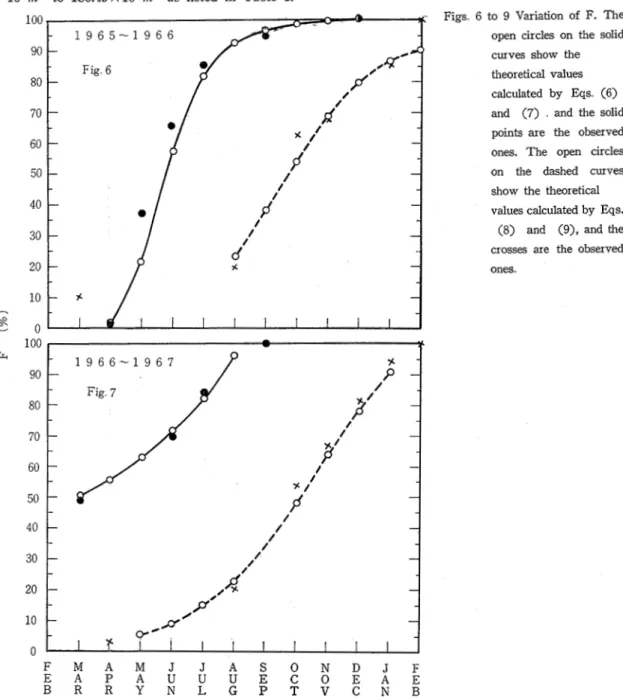
By using Eq. ( 9 , the values of F were obtained as shown in Figs.6 (March 1965 to February 1966), 7 (March 1966 to Febr uaryl967), 8 (March 1967 to February 1968), and 9 (the average of the three years). The solid circles show the values of F for f in the+region or the cumulative values of f in the+ region, and the crosses show the values of F for

f

in the-region or the

Figs. 2 to 5 Variation of f The opencir cles show the theoretical values calculated by Eqs (3) and (4), and the solid points are observed ones

M A M J J A S O N D J F A P A U U U E C O E A E R R Y N L G P T V C N B

130 Tech. Bull. Fac. Agr. Kagawa Univ..

cumulative values of f in the-region. These data of F a r e called the observed data of P hereafter. By using Eq. (7), with these observed data(the solid circles), the values of a, 0, and K were obtained as listed in Table 3. Using the values of a, 0, and K in Table 3, and the observed values of F ( t h e solid circles in Figs. 6 to 9 ) , the values of Ft (theoretical values of F) were obtained by Eq. (6) as shown by the open circleson the solid curve in Figs. 6 to 9. From these graphs, it is plain that the theoretical values of F or Ft are close to the observed ones.

Using the observed date (the crosses) shown in Figs. 6 to 9, the values of K, a, and b were obtained by Eq. (9) as listed in Table 4. By using Eq. (8), with the values of K, a, and b in Table 4 and the values of F (the crosses in Figs. 6 to 9), the theoretical values of F or F' t

were obtained as shown by the open circles on the dashed curve in Figs. 6 to 9. The graphs

M A M J J A S O N D J F A P A U U U E C O E A E R R Y N L G P T V C N B

1701. 20, No. 2(1969) 131 in these figures show that the theoretical values are close to the observed ones throughout the years.

5. Summary

A study was made to estimate the values of aquifer increasing or decreasing during two consecutive months and to find their characteristics by means of a time series analysis. T h e results that were obtained are as follows:

1) The values of aquifer increasing or decreasing during two consecutive months,

dv,

were obtained by Eq. (I), and the results showed that the values of

dv

varied from-158.95X 104m3 to 186.49X 104m3 as listed in Table 1.

Figs 6 to 9 Variation of F. The open circles on the solid curves show the theoretical values calculated by Eqs (6) and (7) and the solid points are the observed ones. The open circles on the dashed curves show the theoretical values calculated by Eqs.

(8) and (9), and the crosses are the observed ones 100

-

Y-

-

1 9 6 6 - 1 9 6 7 90 - /

6

-- 80 - - / /

3'

70 -

-

- 60 - /

8'

- 50 -

-

- / 40 - /

I;'

- / / 30 - _/ / -

-

20 -

4'

- - 10 -

pO'

-

e

N'

0

l

T

l

I I 1 I I I 1 I F M A M J J A S O N D J F E A P A U U U E C O E A E B R R Y N L G P T V C N B

132 Tech.. Bull. Fac. Agr.. Kagawa Univ. 2) T o see the variation of dv during the period (March to February), the term of

f

was defined by Eq. (2), and the results are shown in Figs. 2 to 5. T o show mathematically the variation of f (the curves show the variation of f ) , Eqs. (3) and (4) were constructed by applying the FOURIER series. The theoretical values of f or f t were obtained by using these

equations as shown in Figs. 2 to 5. As shown in these figures, the theoretical values coincided with the observed ones.

3) The values of the cumulative f in the-tregion were obtained by Eqs.(6) and(7) that were constructed by applying the GOMPERTZ curve. Also the cumulative values of

f

in the-region were obtained by using Eqs.(8) and (9) that were constructed by applying the LOGISTIC curve.

F M A M J J A S O N D J F

E A P A U U U E C O E A E

Vol 20, No. 2(1969) 133 Table 1 Values of dv(l04m3) for every month Table 2 Values of the FOURIER coefficients

from March 1965 to February 1968, and the average of them

-

1967

-

1965 1966 1965 Mar. 1965 Mar.. 1966 Mar.. 1967 Mar. 1965

Month to to to to to to to to

1966 1967 1968 1968 Feb. 1966 Feb. 1967 Feb. 1968 Feb. 1968 Feb 0 00 0 00 0 00 0 00 a0 50 000 50.000 50 000 50 000 Mar A P ~ May June July Aug Sept Oct Nov Dec Jan Feb

Table 3 Values of a, 8, and K Table 4 Values of a, b, and K.

-

-Period a! 0 K Period a b K

Mar I;",:

ti966

0 013207 0 35743 99 271 Mar 1965 to Feb 1966 0 169

-

0 2995 94 199 Mar 1966 to

~~b 1967 3 2007 1 09153 95 898 Mar 1966 to Feb 1967 1 2889 - 0 2275 117 986 Mar I;",; t;968 0 31148 0 52306 100 4 Mar 1967 to Feb 1968 0 9591 - 0 1776 138 993 Mar'

1;",t,ti968

0,. 34403 0 57051 101. 29 Mar. 1965 to Feb, 1968 0. 3413

-

0 2821 98 988

The theoretical values obtained by these equations(the open circles) coincided with the observed ones (the solid circles and the crosses) as shown in Figs. 6 to 9.

4) From these results, it can be pointed out that:(a) the variation of the volumes of the aquifer's increase or decrease during two consecutive months shows a non-periodical one that can be represented by the equations that were constructed by applying the FOURIER series; (b) the variation of the cumulative values of

f

in the+region or the cumulative volume of the aquifer's increase during two consecutive months can be shown by the equations constructed by applying the G O M P E ~ T Z curve; and(c) the variation of the cumulative values of f i n the-region or the cumulative volume of the aquifer's decrease during two consecutive months can be shown by the equation constructed by applying the LOGISTIC curve.

6. A c k n o w l e d g e m e n t s

The writers wish to thank to Emeritus Professor Dr. Hitoshi FUKUDA and Professor Dr. Hiroyuki OGATA, both of Tokyo University for their encouragements. A part of the expenditure was defrayed by the research fund of the Ministry of Education..

134 Tech. Bull.. Fac. Agr., Kagawa Univ.

References

(1) CROXTON, F E , and COWDEN, D J : Practical Bwzness Statistzcs, 594-596 Prentice Hall, Inc , Engle Wood Cliffs, N J

(2) FUKUDA K , et a1 : Shallow Groundwater in the Downstream Basin of the Aya River ( I ) , Tech Bull. Fac Agr Kagawa Uuiv

,

29-35, 17(1965)

(3) FUKUDA, K , et a1 : tbbzd (111), dttto 54-69, 18(1966)

(4) FUKUDA, K , et al : A time series analysis on the variation of the belt of fluctuation of shallow ground- water in paddy fields, dztto 20(1968)

*H~%i*mt~,S1-f

b E E f & T & O

Aquifer

0

( # E )

@ , J \ ~ a ) ~ @ ~ = ~ t ~ ~ ~ ~ @ ~ ~ ~ a ~

7J~EBi&5+0 aquifer GS, @ E (38) t@/J\

(38)

%B%@fK

<

9 $.A? t d A 5 @%f

.

%?.bf% m@R%

L

fc@%?IJ (Figs 2-5) G f , T % W i j $ @ ~ @ @ & z q ; TI@@& FOURIER series & H L b, Eq (3) It 1 7 T

5

L w e

2n 2 z 2n

f t = & + a l t o s k - t a 2 c o s 2 k - + t a n t o s n k -

2 m m m

2n

+ b l sin k zt b 2 sin 2k

2"

+

+bn sin nk -

m m m ( 3 )

FOURIER coefficients i f , 12-ordinate scheme &HL .fc harmonic analysis (Eq 4) 1C 2 7 T g & 5 ~ q . (3) R

a

T;+B

L f e a s f g 12,

W ~ N B .

t

a

<

-g

L ~ C (Figs 2-5)

~ % E % ~ T O @ E ~ O $ A B ~ E (%%%) O@%?!JGZ, Eq (6) ii= h 7 T?j? L @ ~ c

F t =Kapt ( 6 )

a , p % ~ o K o @ ~ T , Eq (7) R k q T % & & %/l\BETGf, Q/J\@O$n@@ (%%?3) % E q (8) K a 7 - c

73 L B f c

K

F' = 1 +lo@+ 6t ( 8 )

a, b $ 1 K 0 @ t % , Eq (9) tE1 7 T g & 5 Eq (6) t i G O M P E R ~ Z curve &, Eq (8) CS LOGISTIC curve%, %&L~?&L%?&T&&~ Eq (6) t E q (8) K L 7 T Z t B L f c @ L I B 4 f , % B U @ t k < - - A (Figs 6 - 9 ) Lfc" Eq(3), Eq(6) % l V Eq(8) I%WHRil6iA5&Ot,E~,5

?L$,

c

OB%?,FE% LfcBH0-$42, 2 3 % N % B R B ( % X B %

-

7k3tq, %#I) K 1 7 T g?L

5

c

2 75rT $ fc L

c

RZ

L T U Q & % b T . (Received November 30, 1968)