Yokota type invariants derived from Costantino-Murakami's Invariants (Intelligence of Low-dimensional Topology)

Yokota

type

invariants derived from

Costantino-Murakami’s

Invariants

Atsuhiko

Mizusawa

Waseda

University

This is

a

survey of [4]. In this note,

we define

invariants for colored

oriented

spa-tial graphs

from

Costantino-Murakami’s

invariants

([2]) following the

method

defining

Yokota’s invariants ([7]). We call these invariants Yokota type invariants. Then

we

pro-pose a volume conjecture between the Yokota type invariants and volumes of hyperbolic

polyhedra.

1

Knots and spatial graphs

In this section, we quickly review knots, spatial graphs, the Reidemeister

moves

for

them, the volume conjecture and Yokota’s invariants.

Definition

1.1. $A$ knot is

an

embeddingof

a

circle into the three-sphere. $A$ spatial graph

(a knotted graph) is

an

embedding of

a

graph $(V, E)$ into the three-sphere. Where $V$ is

a set of vertices and $E$ is a set of edges. $A$ plane graph is

a

spatial graph which

can

be

embedded to the two-sphere.

We treat them through diagrams derived by regular projections to the two-sphere.

Figure 1: Diagrams ofa knot, aspatial graph and a plane graph.

There

are

5local

moves

called Reidemeister

moves

for knot and spatial graph diagrams (Figure 2). Here RIV and $RV$

moves

appear only for spatial graph diagrams.

Theorem 1.2. Two diagrams represent the same knot or spatial graph

_if

and only

_if

the

$-\}_{1}^{)}($

RI RII RIII

RIV RV

Figure 2: Reidemeister moves.

Fkom Theorem 1.2, values or properties derived from diagrams of knots (resp. spatial

graphs) that do not change under the Reidemeister moves are invariants of knots (resp.

spatial graphs).

The $N$-th colored

Jones

polynomial $J_{N}$(. ;q) is

an

invariant for knots

defined

through

an

$N$

-dimensional

representation of_quantum

group

$\mathcal{U}_{q}(sl_{2})$

.

When $N=2$, it corresponds

to the Jones polynomial.

Conjecture 1.3 (Volume conjecture [3] [5]). Let $K$ be a hyperbolic knot in $S^{3}(i.e$

.

the

complement

_of

$K$ has a complete hyperbolic structure). Then the value

of

_{the colored}

Jones polynomial

_of

$K$ at $N$-th root

of

unity $\exp(2\pi\sqrt{-1}/N)$ in the next

form

converges

to the hyperbolic volume

_of

complement

_of

$K.$

$2 \pi\lim_{Narrow\infty}\frac{\log|J_{N}(K;\exp(2\pi\sqrt{-1}/N))|}{N}=Vol(S^{3}\backslash K)$_,

where $Vol(\cdot)$ is the hyperbolic volume.

The volume conjecture is generalized for any knots by using the simplicial volume

(Gromov norm) instead ofthe hyperbolic volume ([5]).

In [7], Y.

Yokota defined

invariants for coloredspatial graphs. $A$ color is

a

non-negative

integer added to the graph edges. The colors correspond to the dimension of the

repre-sentation of$\mathcal{U}_{q}(sl_{2})$

.

$A$ triple $(i, j, k)$ of colors is called admissible (for this representation)

if they satisfy $|i-j|\leq k\leq i+j$ _and $i+j+k\in 2\mathbb{Z}$. Yokota’s invariants

are

first defined

for trivalent graphs then generalized for any graphs.

Definition 1.4 (Yokota’s invariants). Let $\Gamma$ be a trivalent spatial graph. We add colors

to edges of $\Gamma$ such that

diagram $D$of admissibly

colored

$\Gamma$

can

be estimated

by the

Kauffman

bmcket

$\langle\cdot\rangle$ (see

[7]

for details). We put $\Delta_{a}=$

$(i,j, k)$

.

Yokota’s invariants $\langle\cdot\rangle_{Y}$ for colored trivalent graph $\Gamma$

are

defined

as

$\langle\Gamma\rangle_{Y}=\langle D\rangle\langle\overline{D}\rangle/\prod_{Trip1es}$

of

$\theta(i, j, k)$, colors at vertices

wher$e^{}$

means

the

mirror image

of

a

diagram.

Yokota’s invariants

are

generalized

for

spatial graphs which have 1, 2, $n$-valent $(4\leq n)$ verticeswith the next relations at vertices.

for

an

$n$-valent vertex $(4\leq n)$ where color $i$

moves

all admissible colors for the right-hand

side diagram. This relation is independent of the ways extending the edge.

$\langle\frac{i\wedge j}{\vee}\rangle_{Y}=\frac{\delta_{ij}}{\triangle_{i}}\langle\underline{i}\rangle_{Y}$

for

a

2-valent vertex, and

for

an

1-valent vertex.

2

Costantino-Murakami’s invariants

In this section

we

review the invariants for colored oriented framed trivalent spatial

graphs

defined

by F.

Costantino and J.

Murakami in [2].

Here

trivalent graphs

may

have

circle components. These invariants have properties of the volume conjecture between

tetrahedron graphs and hyperbolic volumes oftetrahedra.

2.1 Definition of CostantinoMurakami‘s invariants

Costantino-Murakami’s invariants

are

defined through the non-integral representations

of the quantum group $\mathcal{U}_{q}(sl_{2})$ where $q$ is at a root of unity. $\mathcal{U}_{q}(sl_{2})$ is the Hopf algebra

Generators:

$E,$ $F,$ $K,$ $K^{-1}.$

Relations: $[E, F]= \frac{K^{2}-K^{-2}}{q-q^{-1}},$ $KE=qEK,$ _{$KF=q^{-1}FK,$ $KK^{-1}=K^{-1}K=1.$}

Structure

of the Hopf algebra:

$\triangle(E)=E\otimes K+K^{-1}\otimes E,$ $\triangle(F)=F\otimes K+K^{-1}\otimes F,$ $\triangle(K^{\pm 1})=K^{\pm 1}\otimes K^{\pm 1},$

$S(E)=-qE, S(F)=-q^{-1}F, S(K)=K^{-1},$

$\epsilon(E)=\epsilon(F)=0, \epsilon(K)=1,$

where $\Delta$ is the coproduct, _$S$

is the antipode and $\epsilon$ is the counit.

Let $n\in \mathbb{N}$ and $\xi_{n}$ be

a

$2n$-th primitive root of unity _{$\exp(\pi\sqrt{-1}/n)$}

.

We prepare notations:

$\{a\}=\xi_{n}^{a}-\xi_{n}^{-a}(a\in \mathbb{C}) , [a]=\frac{\{a\}}{\{1\}}, \{k\}!=\prod_{j=1}^{k}\{j\}(k\in \mathbb{N})$,

$\{\begin{array}{l}ab\end{array}\}=\prod_{j=0}^{a-b-1}\frac{\{a-j\}}{\{a-b-j\}} (a, b\in \mathbb{C} s.t. a-b\in\{0,1, \ldots, n-1\})$.

For each non-half-integer complex number $a \in \mathbb{C}\backslash \frac{1}{2}\mathbb{Z}$, there is a simple _$n$-dimensional

representation of$\mathcal{U}_{\xi_{n}}(sl_{2})$

on

a

representation space $V^{a}$ which is

an

$n$-dimensional vector

space whose basis is $\{e_{0}^{a}, \ldots, e_{n-1}^{a}\}$

.

The actions of this representation are given by

$E(e_{j}^{a})=[j]e_{j-1}^{a}, F(e_{j}^{a})=[2a-j]e_{j+1}^{a}, K(e_{j}^{a})=\xi_{n}^{a-j}e_{j}^{a} (e_{-1}^{a}=e_{n}^{a}=0)$.

For two complex numbers $a,$ $b \in \mathbb{C}\backslash \frac{1}{2}\mathbb{Z}$, the two representations related to them

are

isomorphic if and only if $a-b\in 2n\mathbb{Z}$. The dualrepresentation on $(V^{a})^{*}$ is isomorphic to

the representation

on

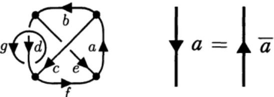
$V^{n-1-a}.$

Let $\Gamma$ be

an

oriented

framed trivalent graph. We add non-half-integercomplex numbers

to each oriented edge of $\Gamma$ (Figure $31eft$

). The numbers are called colors. In the

cal-culations of

Costantino-Murakami’s

invariants (see below), an $a$ colored downward edge

corresponds to the representation space $V^{a}$ and

an

$a$ colored upward edge corresponds to

the dual space $(V^{a})^{*}$. From the isomorphism between the representations on $(V^{a})^{*}$ and $V^{n-1-a}$, we can identify an $a$ colored edge and

$n-1-a$

colored opposite direction edge

(Figure 3 right). We put $\overline{a}=n-1-a$

.

We define admissible _condition for the colors of

$\}a=\}\overline{a}$

Figure 3: $A$ colored oriented trivalent graph (left) and identification of colored edges (right).

Definition 2.1 (Admissible condition). If three colors $a,$$b,$$c$ ofedges at

a

vertex satisfy

the next condition, the triple $(a, b, c)$ of the colors is called admissible.

$a+b+c\in\{n-1, n, \ldots, 2n-2\},$

here the orientations of the three edges

are

all toward the vertex.

If three colors of

a

vertex

are

admissible,

we

can

give

a

representation canonically at

the vertex.

From

now

on, unless otherwise noted, variable colors in summations $\sum$

move

all admissible colors.

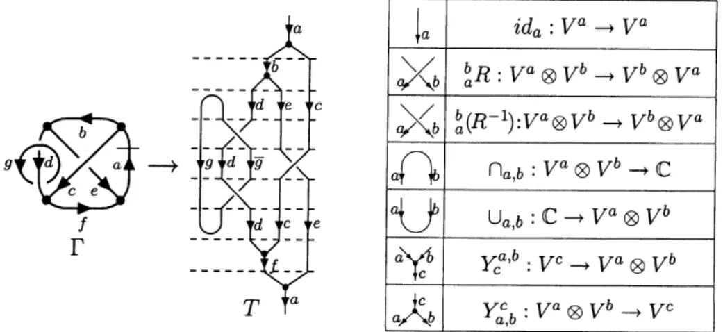
To calculate Costantino-Murakami’s invariants for admissibly colored oriented framed trivalent spatial graph $\Gamma$,

we

cut

an

edge of $\Gamma$ and make an (1, 1)-tangle diagram $T$

so

that the boundary edges of$T$

are

oriented downward. Then

we

cut $T$ to slices

so

that

in each slice there is just

one

singular point, which is

a

maximal, minimal, crossing or

vertex point (Figure 4 left). $A$ boundary of

an

$a$ colored strand in

a

slice is related to

the representation space $V^{a}$ if the strand isoriented downward and to $(V^{a})^{*}$

or

$V^{n-1-a}$ if

the strand is oriented upward. From the representation of$\mathcal{U}_{\xi_{n}}(sl_{2})$, each slice is regarded

as a

map from the tensor product ofrepresentation spaces corresponding to the bottom

boundary

of

strands in the

slice

to the

one

corresponding to the

upper

boundary (Figure

4 right). Here the maps

are

defined

as

follows.

$baR(e_{i}^{a} \otimes e_{j}^{b})=\sum_{m}\{m\}!\xi_{n}^{2(a-i)(b-j)-m(a-b-i+j)-\frac{m(m+1)}{2}}\{\begin{array}{ll}i i- m\end{array}\} \{\begin{array}{l}2b-j2b-j-m\end{array}\}e_{j+m}^{b}\otimes e_{i-m}^{a},$

where $m \in[0, \min(i, n-j-1)]\cap \mathbb{N}.$

$\bigcap_{a,b}(e_{i}^{a}\otimes e_{j}^{b})=\delta_{b,n-1-a}\delta_{i,n-1-j}\xi_{n}^{-(a-i)(n-1)},$ $\bigcup_{a,b}=\delta_{b,n-1-a}\sum_{i=0}^{n-1}\xi_{n}^{-(a-i)(n-1)}e_{i}^{a}\otimes e_{n-1-i}^{b}.$

Figure 4: $\Gamma$ and _$T$ (left),

the maps related to the singular points (right).

where

$C_{i,j,k}=\sqrt{-1}^{c-a-b}(-1)^{j-k}\xi\{\begin{array}{l}2c2c-k\end{array}\}\{\begin{array}{l}2c-(n-1)a+b+c\end{array}\}$

$\sum_{z+w=k}(-1)^{z}\xi\frac{(2z-k)(2c-k+1)}{n2}\{\begin{array}{l}a+b-ci-z\end{array}\}\{\begin{array}{lll}2a -i+ z2a -i \end{array}\} \{\begin{array}{l}2b-j+w2b-j\end{array}\}$

Then

we

have a map $op(T)$ from the representation space related to the _color, say $a,$

of the cutting edge of $\Gamma$ to itself by composing the maps related to the slices of

$T$;

$op(T)$ : $V^{a}arrow V^{a}$. By Schur’s lemma, _$op(T)$ is equal to a scalar $\lambda(T)(\in \mathbb{C})$ multiplied

identity $\lambda(T)id_{a}$

. Costantino-Murakami’s

invariants $\langle\cdot\rangle_{CM}$ of $\Gamma$

are

defined by

$\langle\Gamma\rangle_{CM}=\lambda(T)\{\begin{array}{l}2a+n2a+1\end{array}\}$

Theorem 2.2 ([2]). For colored oriented

_framed

trivalent spatialgraph$\Gamma$, the value $\langle\Gamma\rangle_{CM}$

does not depend

on

the choice

_of

the cutting edge and (1,1)-tangle diagram T.

_Therefore

$\langle\cdot\rangle_{CM}$ is

an

invariants

for

colored oriented

framed

trivalent spatial graph.

Remark 2.3. 1. For

a

half-integer $a \in\frac{1}{2}\mathbb{Z},$

$\{\begin{array}{l}2a+n2a+1\end{array}\}=0.$

Hence for half-integer colors,

Costantino-Murakami’s

invariants may become infinity.

2. If graphs

are

restricted to links,

Costantino-Murakami’s

invariants correspond to

the Akutsu-Deguchi-Ohtsuki (colored Alexander) invariants. For the

Akutsu-Deguchi-Ohtsuki _{invariants, the properties of the volume conjecture between links and cone}

2.2 Relations of Costantino-Murakami’s

invariants

In this subsection,

we

review relations of

Costantino-Murakami’s invariants.

Using the

relations,

Costantino-Murakami’s

invariants

are

calculated axiomatically.

The $6j$-symbols $\{\cdot\}$

are

thevalues determined by 6 colors. The $6j$-symbols

are

defined

as coefficients of the relation (3) below. For $a,$$b,$ $c,$$d,$ $e,$$f \in \mathbb{C}\backslash \frac{1}{2}\mathbb{Z}$ and $a+b-c,$$a+f-$

$e,$$b+d-f,$$d+c-e\in \mathbb{Z}$, the $6j$-symbols

are

calculated by the next formula.

$\{\begin{array}{lll}a b cd e f\end{array}\}=(-1)^{n-1+B_{afe}}\{\begin{array}{l}2f+n2f+1\end{array}\}\frac{\{B_{dce}\}!\{B_{abc}\}!}{\{B_{bdf}\}!\{B_{afe}\}!}\{\begin{array}{lll} 2c A_{abc} +1- n\end{array}\} \{\begin{array}{l}2cB_{{\oe} d}\end{array}\}$

$\cross\sum_{z=s}^{S}(-1)^{z}\{\begin{array}{ll}A_{afe} +12e+z +1\end{array}\} \{\begin{array}{l}B_{aef}+zB_{aef}\end{array}\}\{\begin{array}{l}B_{bfd}+B_{dce}-zB_{bfd}\end{array}\}\{\begin{array}{l}B_{dec}+zB_{dfb}\end{array}\},$

where $s= \max(0, -B_{bdf}+B_{dce}),$ $S= \min(B_{doe}, B_{afe}),$ $A_{xyz}=x+y+z,$ $B_{xyz}=x+y-z.$

Costantino-Murakami’s invariants of tetrahedron graphs

are

described by using the

6j-symbols and

we

denote them by $\{\cdot\}_{tet}.$

$\{\begin{array}{lll}a b cd e f\end{array}\}.$

It

was

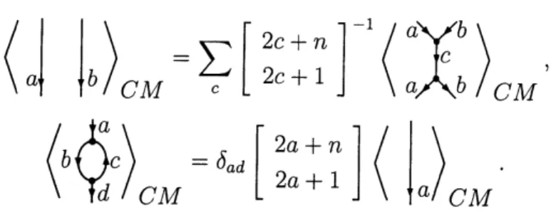
proved that $\{\cdot\}_{tet}$ is well-defined for half-integer colors. The next local relations

hold for Costantino-Murakami’s invariants.

$\langle\rho^{1_{a}}\rangle_{CM^{=\xi_{n}^{-2a\overline{a}}}}\langle 1_{a}\rangle_{CM} \langle\}ab\rangle_{CM}=\xi_{n}^{2a\overline{a}}\langle 1_{a}\rangle_{CM}$ (1)

(2)

$b$

(3)

$d$

$\langle_{a}\downarrow$ _{$\downarrow b\rangle_{CM}=\sum_{c}$}

$l_{a}\rangle_{CM}$

2.3 Properties of the volume conjecture

Costantino-Murakami’s

invariants

have properties of the volume conjecture

between

tetrahedron _{graphs and hyperbolic volumes of ideal and truncated tetrahedra (Figure 5}

left). Shapes of tetrahedra in the hyperbolic space are determined by their 6 dihedral

angles of edges. The ideal tetrahedra are the hyperbolic tetrahedra whose vertices are

all at infinity points of hyperbolic space. The two dihedral angles of opposite edges of

ideal tetrahedra

are

equal. _{Therefore the shapes of ideal tetrahedra}

_are

_{determined by}

3 dihedral angles $\alpha,$$\beta,$

$\gamma$

.

It is known that they satisfy $\alpha+\beta+\gamma=\pi$

.

In the Klein model of hyperbolic space,

we

can consider the tetrahedron whose vertices

are

“outside”

the hyperbolic space (Figure 5 right). For each vertex of this tetrahedron, there is just

one

geodesic _{surface which intersects perpendicularly to each of three adjacent faces of}

the vertex. _{Cutting the tetrahedron by the surfaces at} every vertex,

we

have

a

finite

polyhedron in the hyperbolic space. This polyhedron is called truncated tetrahedron.

Three dihedral angles $\alpha,$$\beta,$

$\gamma$of edges adjacent toan “outside” vertex satisfy $\alpha+\beta+\gamma<\pi.$

Klein Model Poincar\’e Model

Figure 5: Images of ideal and truncated tetrahedra(left), a vertex outside the hyperbolic space and a cutting surface (gray) (right).

Theorem 2.4 ([2]). Let $S$ be a hyperbolic tetmhedron, $\theta_{a},$

$\cdots,$$\theta_{f}$ be dihedml angles

of

$S$ and $a_{n},$$\cdots,$$f_{n}$ be sequences

of

integer colors such that _{$\lim_{narrow\infty}\frac{2\pi a}{n}=\pi-\theta_{a},$}$\cdots$ $\lim_{narrow\infty}\frac{2\pi f_{n}}{n}=\pi-\theta_{f}$

.

Costantino-Murakami’s

invariants

of

tetmhedron graphs _{$\{\cdot\}_{tet}$}

($i.e$

.

dihedml

angles

of

opposite edges

are

equal),

$Vol(S) =\lim_{narrow\infty}\frac{\pi}{n}\log((-1)^{n-1}\{\begin{array}{lll}a_{n} b_{n} c_{n}a_{n} b_{n} c_{n}\end{array}\})$

$= \lim_{narrow\infty}\frac{\pi}{n}\log((-1)^{n-1}\{\begin{array}{l}\overline{a_{n}}\overline{b_{n}}\overline{c_{n}}\overline{a_{n}}\overline{b_{n}}\overline{c_{n}}\end{array}\})$

If

$S$ is

a

truncated tetmhedmn,

$Vol(S)=\lim_{narrow\infty}\frac{\pi}{2n}\log(\{\begin{array}{lll}a_{n} b_{n} c_{n}d_{n} e_{n} f_{n}\end{array}\} \{\overline{\frac{a_{n}}{d_{n}}}\overline{\frac{b}{e_{n}}n}\overline{\frac{c_{n}}{f_{n}}}\}_{tet})$

.

(5)

3

Yokota

type

invariants

and numerical calculations

In this section,

we

define Yokota type invariantsfor coloredoriented spatial graphs with

more

than

or

equal to 3-valent vertices from Costantino-Murakami’s invariants. We also

propose

a

volume conjecture for the Yokota type invariants between plane graphs and

hyperbolic

convex

tetrahedra. By numerical calculations,

we

observe regularities of the

Yokota type invariants for integer colors and asymptotic behaviors ofthem.

3.1 Definition of Yokota type

invariants

Using the similar way to define Yokota’s invariants, Costantino-Murakami’s invariants

are generalized to invariants for non-framed colored oriented spatial graphs with

more

than or equal to 3-valent vertices. Like the Yokota$\rangle s$ invariants, these invariants are first

defined for trivalent graphs thengeneralized for graphswith

more

than 3-valrent vertices.

Definition

3.1 (Yokota type invariants). Let $\Gamma$ be admissibly colored oriented trivalent graph and $D$ be its diagram. Yokota type invariants $\langle\cdot\rangle_{Y}$,

are

defined from

Costantino-Murakami’s invariants by the next relation.

$\langle\Gamma\rangle_{Y’}=\langle D\rangle_{CM}\langle\overline{D}^{r}\rangle_{CM},$

wher$e^{}$ means the mirror image, $\cdot$

$r$

means

reversing orientations ofall edges. Using the

next relation, we define the Yokota type invariants for graphs with more than 3-valent

vertices.

where the surrounding edges have the

same

colors and orientations on the both sides and

Theorem 3.2. The values

_of

the Yokota type invariants

are

independent

_of

the choice

_of

the diagrams to calculate and

_of

the ways to extend edges at

more

than 3-valent vertices.

Pmof.

This is

a

sketch ofproof. Theinvariance ofthe Yokota type invariantsfor RII, RIII

and$RV$

moves

come

from that of

Costantino-Murakami’s

_{invariants. The invariance for$RI$}

and RIV

moves come

from direct calculations using the relations (1) and (2) respectively. The next equation holds for the Yokota type invariants.

By extending edges at a

more

than 3-valent vertex recursively, it changes to a trivalent

tree. The shape ofthe tree depends on the ways to extend the edges. The values of the

result graphs are, however, the

same

because the trees

are

transformed to each other by

a

sequence of the

moves

in the equation. $\square$

In Theorem 2.4, the value inside log$(.$ $)$ of Equation (5) is the value ofthe Yokota type

invariants for tetrahedron graphs. Using the Yokota type invariants, we conjecture the

extension of Theorem 2.4.

Conjecture

3.3.

Let$\Gamma$ be

a

plane graph

and

$S_{\Gamma}$ be

a

hyperbolic

convex

polyhedmn which

is bounded by $\Gamma$.

If

sequences

_of

integer colors

_of

$\Gamma$ are taken as in Theorem

2.4 for

corresponding dihedral angles

_of

$S_{\Gamma}$, then

$Vo1(S_{\Gamma})=\lim_{narrow\infty}\frac{\pi}{2n}\log(\langle\Gamma\rangle_{Y’})$ .

3.2 Numerical calculations

We show the numerical calculations of the Yokota type invariants for square pyramid

graphs andobserveregularities of the Yokota type invariantsfor integer colors and

$= \sum_{i}\{\begin{array}{ll}2i+ n2i+1 \end{array}\} \{\begin{array}{lll}a e di c b\end{array}\}\{\begin{array}{lll}d g hf c i\end{array}\} \{\begin{array}{l}\overline{a}\overline{e}\overline{d}\overline{i}\overline{c}\overline{b}\end{array}\}\{\begin{array}{l}\overline{d}\overline{g}\overline{h}\overline{f}\overline{c}\overline{i}\end{array}\}$

where the thirdequation

uses

therelation (4). Weconsidercolored squarepyramidgraphs

$\Gamma_{1,n}$ and $\Gamma_{2,n}$ corresponding to the followingsquare pyramids.

where all vertices of the squarepyramid of$\Gamma_{1,n}$

are

truncated and the4 bottomverticesof

the square pyramid of$\Gamma_{2,n}$

are

ideal vertices. The sequences of colors become integers by

taking appropriate integer $n$. For the integral colors, the

formula of

the

square

pyramid

graph looks diverging to infinity because of the coefficient $\{\begin{array}{ll}2i+ n2i+1 \end{array}\}$ and

even

the

regularity at the integer colors of the square pyramid formula is not proved yet. When

we

do numerical calculations,

we

slightly differ the integer colors using small real number $\epsilon$ preserving admissible conditions.

Before the numerical calculations,

we

show algebraic computation ofthe formula ofthe

squarepyramids. Wecalculated the formula

as a

rationalfunction of$q$by not substituting

$\xi_{n}$ to _$q$ (i.e. defining $\{a\}=q^{a}-q^{-a}$) and reduced the numerator and the denominator by

common

factors then substituted $q=\xi_{n}$

.

The results

are as

follows.

$\Gamma_{1,n}:n=24,$ $\{a, b, c, d, e, f, g, h\}=$

{9,8,9,9,8,8,8,9},

$\frac{2702553921462776104873773262573943868288}{4144454025633775}.$

$\Gamma_{2,n}:n=12,$ $\{a, b, c, d, e, f, g, h\}=$

{4,4,4,4,4,4,4,4},

$\Gamma_{2,n}:n=24,$ $\{a, b, c, d, e, f, g, h\}=$

{8,8,8,8,8,8,8,8},

$\frac{1841727671678193906056765234366258287027200}{19743796020815679008287}.$

The values are finite and the regularities for these $n$’s

are

shown. However, the above

computation for large $n$ takes too long time.

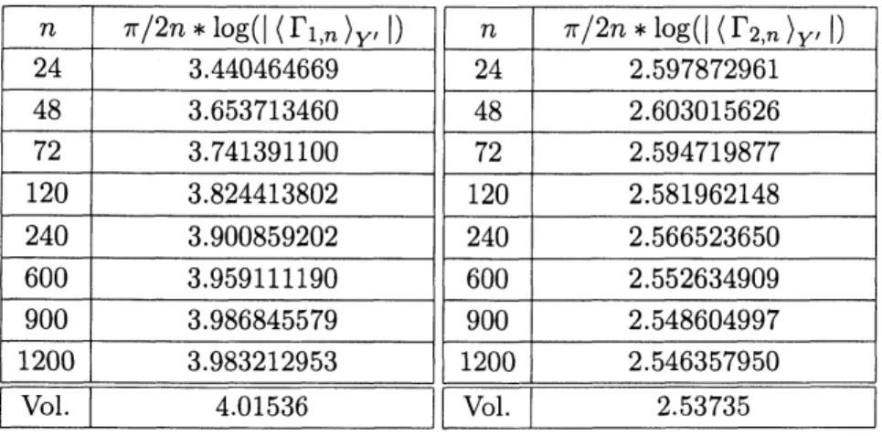
We

did numerical calculations at $\epsilon=$

0.0000001

and observed asymptotic behavior ofthe formulafor $\Gamma_{1,n}$ and $\Gamma_{2,n}$. The results

are

in Table 1, where

we

calculated to 9th decimal places. We took the absolute values

of the Yokota type invariants to kill the multivalency of $\log$ because in the result of the

calculations the value of Yokota type invariant for each $n$

was

a negative real number.

We need

more

discussions here. The results

seem

to tend to the volume of each square

Table 1: Numerical calculations at $\epsilon=0.0000001$

pyramid. These near-integer colors calculations also show that the formula may have

regularities at integer colors. The results are not so strong supporting evidences for Conjecture 3.3. We propose the next problem.

Problem 3.4. Pmve Conjecture 3.3

_for

some

polyhedm which have

more

than 3-valent

vertices. References

[1] J. Cho and J. Murakami Some limits

_of

the coloredAlexander invariant

_of

the figure-eight knot and the volume

_of

hyperbolic orbifolds, J. Knot Theory Ramifications 18

no.

9 (2009), 1271-1286.

[2] F. Costantino and J. Murakami On $SL(2,$C) quantum $6j$-symbol and its relation to

[3]

R.

Kashaev The

hyperbolic

volume

_of

knots

_from

the quantum dilogarithm,

Lett,

Math. Phys. 39 (1997),

269-275.

[4] A. Mizusawa and J. Murakami Yokota Type Invariants Derived

_from

Non-integml

Representation

_of

$\mathcal{U}_{q}(sl2)$, in preparation.

[5] H. Murakami and J.

Murakami

The colored

Jones

polynomials and the simplicial

volume

_of

a

knot,

Acta

Math. 186

no.

1 (2001),

85-104.

[6] J. Murakami Colored Alexander invariant

_for

_framed

links, Osaka J. Math. 45

no.

2

(2008), 541-564.

[7] Y. Yokota Topological invariants

_of

graphs in 3-space, Topology 35 (1996), 77-87.

Department of Mathematics

Waseda University Tokyo

169-8050

JAPAN

$E$-mail address: a-mizusawa @aoni.waseda.jp