Filtering volatility from data observed at random time intervals(The 7th Workshop on Stochastic Numerics)

Filtering volatility from

data

observed at

random

time

intervals

Jaksa

Cvitanie

*

Robert

Liptser

\dagger

Boris

Rozovskii

\ddagger

Ilya Zaliapin

\S

October 10,

2005

$AMS$ (2000) Subject

Classifications:

Primaxy $60\mathrm{G}35,91\mathrm{B}28$; secondary $62\mathrm{M}20,93\mathrm{E}11$.

Key Words and Phrases: nonlinear filtering, discrete observations, volatility estimation.

Abstract

Weconsideracontinuous-time model forastockprice,whichis, however, observed at discrete time intervals. The time between observations is random. Wereportonthe formula for the optimal filter for the current value of the volatility of the stock price and we illustrate the theoretical results with a numerical example. The filter gives

stable and efficient estimates of thevolatility As apreliminary step, we estimate the possible values of volatilityusinga variation of the Multiscale Trend Analysis (MTA) method.

*Caltech, $\mathrm{M}/\mathrm{C}$ 228-77, 1200 E. California Blvd. Pasadena, CA 91125. Ph: (626) 395-1784. $\mathrm{E}$mail:

[email protected]. Researchsupported inpart by NSF grant DMS 04-03575.

$\uparrow \mathrm{D}\mathrm{e}\mathrm{p}\mathrm{a}\mathrm{r}\mathrm{t}\mathrm{m}\mathrm{e}\mathrm{n}\mathrm{t}$ of Electrical Engineering-Systems, Tel Aviv University, 69978 Tel Aviv, Israel.

E-mail:[email protected]

tDepaxtment ofMathematics , USC, 3620 $\mathrm{S}$Verm ont Ave, MC 2532, Los Angeles, CA90089-1113, Ph:

(213) 740-6117, $\mathrm{E}$-mail: [email protected]. Researchsupported in part bythe ArmyResearch Officeand

the Office ofNavalResearchunderthe grants DAAD19-02-1-0374 and N0014-03-0027.

InstituteofGeophysics and PlanetaryPhysics,UCLA, 3845SlichterHall, Los Angeles, CA90095-1567,

2

1

INTRODUCTION

Inthispaper

we

report

on

theoretical results fromCvitanic, Liptserand Rozovskii [3] andon theirnumericalimplementation inCvitanic’, Rozovskii andZaliapin [4]. Theproblem

we

con-sider is the one of estimating the current volatility value from stock priceobservations. The observations

are

discrete, possiblyobserved at random times. The mainapplication

we

have in mind is high-frequency stock data (”tick-by-tick” data).

We

work in

a

continuous-time, Brownian motiondriven model for the stock price, with stochastic volatility, independent of the driving Brownian motion

process.

Related literature includes, among others, Prey and Runggaldier [7], Runggaldier [25], Elliott et al [5], Gallant and

Tauchen

[8], Malliavin and Mancino [20], Fouque et al. [6], Rogers and Zane [23], and Kallianpur and Xiong [13], Ait Sahaliaand Mykland [1], Platania and Rogers [22], andJohannes andPoison [11]. Thereis also arich econometrics, time-series literature on ARCH-GARCH mod els of stochastic volatility, presenting

an

alternative way to model and estimate volatility;

see Gourieroux

[9] for

a

survey.

Our work

was motivated

primarily by Prey and Runggaldier [7]. That paper derives

a

Kallianpur-Striebel type formula (see e.g. [12]) for the optimal mean-square filter of the volatility process, and investigates Markov Chain approximations for this formula. We extend this result in that

we

derive the exact filtering equations, which

can

easily be imple-

mented-The Prey and Runggaldier model is anatural model for stochastic volatility, but it does not quite fall in the “standard” category of diffusion

or

simple point processes models for which filtering results have been developed (cf. [18], [15], [24]). Thus, there

was

a need to develop further technical tools to deal with our problem. However, it turns out that the resulting filtering equations

are

simplerthan in the

case

ofcontinuous

observations.

In the latter case, the nonlinear filters are described by infinite dimensional stochastic differential equations, for example, by stochastic partial

differential

equations (see

e.g.

[24]). In

con-trast, in

our

setting, the filtering equation

can

be reduced to

a

recursive system of linked deterministic equations of Kolmogorov type. Moreover, at the observation times the filter is given by a simple Bayesian recursion.

In

our

numerical example

we assume

th at the volatilityis

a

Markov chainprocess. Before

we can

dothe filtering,

we

have to decide whatpossiblevalues thevolatilitychain

can

attain,

and

what the transition probabilities

are.

This preliminary stage is related to the power variationestimates of volatility,

as

surveyed in Barndorff-Neielsen,

Graversen

and Shephard [2], for example. We adapt the so-called Multiscale

Trend

Analysis of Zaliapin et $al$ $[27]$,

where

we use

a

variation process to estimate possible volatility values. However, while in thepower variations literature such

an

estimate is

the final

estimate ofvolatility, in

our

case

using filtering. Also, let

us

emphasize again that, unlike most of the existing work, the time intervals between observations maybe random in

our

framework.

We show that the complete algorithm, consisting ofthe preliminary estimation and the filtering estimation, performs very well in

a

variety of circumstances,

on

simulated and

on

real data. It quickly recognizes when there $1S\lrcorner$

a

jump in volatility value. It is also robust

with respect to the given drift value, which is important,

as

the drift is hard to estimate in practice,

Wedescribethe modelin section 2,state themain filtering results andexamplesinsection 3, discuss the preliminary estimation of the model parameters in section 4, the numerical implementation of the filtering formula in section 5, and the complete algorithm in section

6.

We

present two examples with real datain section

7.

2

THE

MODEL

2.1

Observation

values and

observation

times

We fix a probability space $(\Omega, \mathcal{F}, \mathrm{P})$ equipped with a filtration $\mathrm{F}$

$=(\mathcal{F}_{t})_{t\geq 0}$ satisfying the

“usual” conditions (see, e.g. [19]). All random

processes

consideredin thepaper are assumed to be defined

on

$(\Omega, \mathcal{F}, \mathrm{P})$ and adapted to F.

We consider astock price process $S=(S_{t})_{t\geq 0}$ given bythe It6 equation

$fS_{t}=r(\theta_{t})\mathit{3}_{t}dt+v(\theta_{t})S_{t}fB_{t}$ (2.1)

where $B=(B_{t})_{t\geq 0}$ is

a

standard Brownian motion and $\theta=(\theta_{t})_{t\geq 0}$ is

a

cadlag Markov

jump-diffusion processin IR withthe generator $\mathcal{L}$

.

For thesake of simplicity,

we

assume

that

$r(x)$ and $v(x)$ are measurable bounded functions

on

$\mathbb{R}$, the initial condition $S_{0}$ is constant,

and $v(x)$ and $S_{0}$ are positive.

The process $(\theta_{t})_{t\geq 0}$ isreferred to

as

the volatilityprocess. It is unobservable,

and

theonly observable quantities

are

the values of the $\log$-price process $X_{t}=\log S_{t}$

taken

at stopping

times $(T_{k})_{k\geq 0}$,

so

that $T_{0}=0$,$T_{k}<T_{k+1}$ if$T_{k}<\infty$, and $T_{k}\uparrow$

oo as

$j_{\acute{v}}\uparrow\infty$

.

According to (2.1), the $\log$-price process is given by

$X_{t}= \int_{0}^{t}(r(\theta_{s})-\frac{1}{2}v^{2}(\theta_{s}))ds+\oint_{0}^{t}v(\theta_{s})dB_{s}$ .

We

use

the abbreviated notation$X_{k}:=X_{T_{k}}$.Thus, the observations

are

given by the sequence

{Tkl$X_{k})_{k\geq 0}$. The observation process $(T_{k}, X_{k})_{k\geq 0}$ is

a

multivariate (marked) point process

(see,

e.g.

[10], [16]) with the counting

measure

4

where $\delta_{\{T_{k},X_{k}\}}$ is the Dirac delta-function

on

$\mathbb{R}_{+}\mathrm{x}$ R.

We introduce two filtrations relatedto $(T_{k}, X_{k})_{k\geq 0}:(\mathcal{G}(n))_{n\geq 0}$ and $(\mathcal{G}_{t})_{t\geq 0}$, where

- $\mathcal{G}(n):=\sigma\{(T_{k}, X_{k})_{k\leq n}\}$,

- $\mathcal{G}_{t}:=\sigma(r([0, s]\mathrm{x} \Gamma)$ : $s\leq t,$$\Gamma\in \mathrm{B}(\mathrm{R})$, where $B(\mathbb{R})$ is the Borel a-algebra

on

R.

It is

a

standard fact (see IIL3.31 in [10])

$\mathcal{G}_{T_{k-}}=\mathcal{G}(k)$, $k=0,1\ldots$ , (2.2)

and $\{T_{k}\}$ is a system ofstopping times with respect to $(\mathcal{G}_{t})_{t\geq 0}$.

Remark 2.1 The filtration $(\mathcal{G}_{t})_{t\geq 0}$ provides

more

information thanthefiltration$\mathcal{G}_{T_{k}}$, namely

it provides additional information about the duration between the observation times,

The paper Cvitanic, Liptser and Rozovskii [3] works out thefiltering

formula for

general observation times, but here, for the simplicity ofpresentation, we will

assume

the following: Assumption 2.1 The observation times $(T_{k})_{k\geq 0}$

are

either:

(i) the jumptimes of a doubly stochasticPoissonprocess (Cox process) with theintensity

$n(\theta_{t})$,

or

(ii) $T_{k}=\mathrm{k}\mathrm{S}$, that is, the observation times

are

deterministic, with constant length

a

of

interarrival intervals.

2.2

Volatility

Process

We

now

specify more preciselythe volatility process. Let $(\mathbb{R}, B(\mathbb{R}))$ and $(\mathbb{R}_{+}\mathrm{x} \mathbb{R},B(\mathbb{R}_{+})\otimes$

$B(\mathbb{R}))$ be measurable spaces with Borel $\mathrm{c}\mathrm{r}$-algebras. The volatility

process

$\theta=(\theta_{t})_{t\geq 0}$ is

defined by the It6 equation

$d \theta_{t}=b(t, \theta_{t})ft+\sigma(t, \theta_{t})dW_{t}+\oint_{\mathrm{R}}u(\theta_{t-\}}x)(\mu^{\theta}-\nu^{\theta})(dt, dx)$, (2.3)

where $W_{t}$ is

a

standard Wiener process and $\mu^{\theta}=\mu^{\theta}(dt, dx)$ is

a

Poisson

measure

on

$(\mathbb{R}_{+}\mathrm{x} \mathbb{R}_{1}B(\mathbb{R}_{+})\otimes B(\mathbb{R}))$ with the compensator $\nu^{\theta}(dt, fx)=K(dx)dt$

, where

$K(dx)$ is a

a-finite non-negative

measure on

$(\mathbb{R}, B(\mathbb{R}))$. We

assume

that $E\theta_{0}^{2}<\infty$

,

the

functions

$b(t, z)_{\gamma}\sigma(t, z)$, and $u(z,x)$

are

Lipschitz continuous in $z$ uniformly with respect to other

variables,

and

$|b(t, z)|+| \sigma(t, z)|^{2}+\int_{\mathrm{J}\mathrm{R}}|u(z, x)|^{2}K(dx)\leq C(1+|z|^{2})$.

It is well known that under these assumptions (2.3) possesses a unique strong solution adapted to $\mathrm{F}$, and _{$E\theta_{t}^{2}<\infty$}

for any

_{$t\geq 0$}.

The generator of the volatility process is given by

$\mathcal{L}f(x):=b(t, x)f’(x)+\frac{1}{2}\sigma^{2}(t, x)f’(x)$

$+ \oint_{\mathbb{R}}(f(x+u(x, y))-f(x)-f’(x)u(x,y))K(fy)$.

Before proceeding with the assumptions and main

results

we shall introduce

additional

notation. Set

$m(s, t)=f_{s}^{t}(r( \theta_{u})-\frac{1}{2}v^{2}(\theta_{u}))$du, (2.4)

and

$\sigma^{2}(s, t)=\int_{s}^{t}v^{2}(\theta_{u})du$ (2.5)

For simplicity, it is assumedthat$v^{2}(s, t)$ isbounded away from zero. Let

us

denote by$\rho_{s,t}(y)$

the density function of the normal distribution with

mean

$m(s, t)$ and thevariance $\sigma^{2}(s, t)|$

.

$\rho_{s,t}(y):=\frac{1}{\sqrt{2\pi}\sigma(s,t)}e^{-\frac{(y-m(s,t)\mathrm{J}^{2}}{2\sigma^{\Xi}(s,t)}}$ (2.6)

Clearly, $\rho$ is the conditional density of the stock’s $\log$-increments $X_{t}-X_{s}$ given $\theta$.

Let $\mathcal{F}^{\theta}=(\mathcal{F}_{t}^{\theta})_{t\geq 0}$ be the right-continuous filtrationgenerated by $(\theta_{t})_{t\geq 0}$ and augmented

by $\mathrm{P}$

-zero

sets bom

F.

Denote by $G_{k}^{\theta}$ a regular version of the conditional distribution of $T_{k+1}$with respect to” $\mathcal{F}^{\theta}\vee \mathcal{G}(k)$. That is, $G_{k}^{\theta}$ is the distribution of the time of the next

observation, given previous history, and given ?.

Let $N=(N_{t})_{t\geq 0}$ be the countingprocess with interarrival times $(T_{k}-T_{k-1})_{k\geq 1}$ , that is

$N_{t}= \sum_{k\geq 1}I(T_{k}\leq t)$ (2.7)

We also

assume

Assumption 2.2 The Brownian motion B is independent of $(\theta,$

N).

3

FILTERING RESULTS

3,1

_{The main result}

For

a

measurablefunction$f$

on

$\mathbb{R}$such that _{$E|f(\theta_{t})|<\infty_{?}$}define the conditional expectation

estimator $\pi_{t}(f)$ by

$\pi_{t}(f):=E(f(\theta_{t})|\mathcal{G}_{t})=f_{\mathbb{R}}f(z)\pi_{t}(dz)$, (3.1) Here and below$\mathcal{F}^{1}\vee F^{2}$ stands for the$\sigma$-algebra generatedby thea-algebras$F^{1}$ and$\mathcal{F}^{2}$

.

$\mathrm{e}$

where $\pi_{t}(dz):=dP(\theta_{t}\leq z|\mathcal{G}_{t})$ is thefilteringdistribution, (Notethat

we

omitthe argument $\theta_{t}$ of_$f$ inthe estimator $\pi_{t}(f))$. As in the Bayesian framework, we suppose that the

a

priori

distribution $\pi_{0}(dx)=P(\theta_{0}\in fx)$ is given.

Let $\sigma\{\theta_{T_{k}}\}$ be the $\mathrm{c}\mathrm{r}$-algebra generated by $\theta_{T_{k}}$. For $t>T_{k}$, let

us

define the following

struc

rure

_functions:

$\psi_{k}(f;t_{7}y, \theta_{T_{k}}):=B(f(\theta_{t})\rho_{T_{k)}t}(y-X_{k})\phi(T_{k}, t)|\sigma\{\theta_{T_{k}}\}\vee \mathcal{G}\tau_{k})$ (3.2)

and its integral with respect to $y$

$\overline{\psi}_{k}(f).t$,$\theta_{T_{k}}):=\int_{\mathbb{R}}\psi_{k}(f;t, y, \theta_{T_{k}})dy=E(f(\theta_{t})\phi(T_{k}, t)|\sigma\{\theta_{T_{k}}\}\vee \mathcal{G}_{T_{k}})$ (3.3)

where $\rho$ is given by $(2,6)$ and

$\phi(t)$ $=$ $\mathrm{n}(9\mathrm{t})\exp(-\int_{T_{k}}^{s}n(\theta_{\mathrm{u}})du)$ if Assumption 2.1 (i) holds (3.4) $\phi(t)$ $=$ 1 if Assumption 2.1 (ii) holds, (3.5)

If $f\equiv 1$, the argument $f$ in $\psi$ and $\overline{\psi}$ is replaced by 1.

For $t\geq T_{k}$ and a bounded function $f$ , define

$\mathcal{M}_{k}(f;t, \pi_{t}):=\cdot\frac{\pi_{T_{k}}(\overline{\psi}_{k}(f,t))-\pi_{t-}(f)\pi_{T_{k}}(\overline{\psi}_{k}(1\cdot t))}{\int_{t}^{\infty}\pi_{T_{k}}(\overline{\psi}_{k}(1\cdot s))ds}.,’$.

The main filtering result from Cvitanic, Liptser and Rozovskii [3] is (specialized to

As-sum

ption 2.1):

Theorem 3.1 Under

our

assumptions,

_for

every measurable bounded

_function

$f$ in the

do-main

_of

the generator $\mathcal{L}$ such that $\int_{0}^{t}E|\mathcal{L}f(\theta_{s})|ds<$

oo

for

any $t\geq 0$, thefollowing system

of

equations holds:

1) For every $k=0$_,1 $\ldots$ , at the observation times vie have

$\pi_{T_{k+1}}(f)=\frac{\pi_{T_{k}}(\psi_{k}(f,t,y))}{\pi_{T_{k}}(\psi_{k}(1\cdot t,y)\rangle},\cdot|$

$\{\begin{array}{l}t=T_{k+1}y=X_{k+1}\end{array}\}$

(3.6)

Under Assumption 2.1 (i);

we

have between observation times: 2) For

every

$k=0,1$

.

,

.

and $t\in \mathrm{Q}T_{k},T_{k+1}[$,

$f\pi_{t}(f)=\pi_{t}(\mathcal{L}f)dt$ -$\mathcal{M}_{k}$$(f;t_{\}\pi_{t})$

it.

(3.7)

Under Assumption 2.1 (ii), the second $tem$ is zero, that is,

we

have:

2) For every $k=0$, 1$\ldots$ and$t\in \mathrm{I}T_{k}$,$T_{k+1}[$

,

Remark 3,1 _{Note that for high-frequency observations, it maybe satisfactory to compute}

the volatilityestimate only at price observationtimes. In that

case

we only need to

use

the relatively simple Bayes-type recursion formula (3.6), and not the differential equation (3.7)

or

(3.8).

Remark 3.2 Clearly, the “structure functions” $\psi$ and $\overline{\psi}$

are

of paramount importance

for

computingthe posterior distribution ofthe volatility process. We would like to stress that these do not involve the observations and could be pre-computed “$\mathrm{o}\mathrm{f}\mathrm{f}- 1\mathrm{i}\mathrm{n}\mathrm{e}^{1}$’ using only the

a

prioridistribution. Then, “on-line”} when the observations becomeavailable,

one

needsonly

to plug in the

obtained

measurements $(T_{k}, X_{k})$

.

This is important for developing

efficient

numerical algorithms.

Remark 3.3 Note that for almost

every

$\omega$ $\in\Omega$, filtering equation (3.7) is a deterministic

equationofKolmogorov’s type, rather then

a

stochasticpartialdifferentialequationarising in nonlinearfilteringof diffusion

processes.

Thewell-posedness andregularityofsuchequations iswell

researched

in theliterature

on

second orderparabolicdeterministic integro-differential equations (see e.g. [17]i, [21], [14] and the references th erein),

3.2

The

case

of

the Markov

chain

volatility

process

In this section we specialize

our

formulas to the

case

wherethe volatilityprocess is modeled by a continuous time Markov chain.

We

assume

that the counting process is

a

Cox

process

with in tensity $n(\theta_{t})$, and that

$\theta=(\theta_{t})_{t\leq T}$ is a homogeneous Markovjump process taking values in the finite alphabet $A=$

$\{a_{1}, \ldots, a_{M}\}$ with the intensity matrix $\mathrm{A}=(\lambda(a_{\dot{\mathrm{z}}}, a_{j}))=(\lambda_{ij})$ and the initial distribution

$p_{q}=P(\theta_{0}=a_{q})_{:}$ $q=1$, $\ldots$ $\mathrm{J}$M. (Thisis

one

of thetwomodels of the state process discussed

in [7].) In this case,

$\mathcal{L}f(\theta_{s})=\sum_{J}\lambda(\theta_{s}, a_{j})f(a_{j})$

Denote by $\theta_{t}^{j}$ the process $\theta_{t}$ starting from

$a_{j}$, and

$p_{ji}(t):=P(\theta_{t}=a_{i}|\theta_{0}=a_{j})$ , $\pi_{j}(t)=P(\theta_{L}=a_{j}|\mathcal{G}_{t})$ ,

$r_{ji}(t, z):=E(e^{-\int_{0}^{\mathrm{t}}n(\theta_{u}^{j})du}\rho_{0,t}^{?}(z)|\theta_{t}^{j}=a_{i})\}$

where $\rho_{0,\mathrm{r}}^{J}(z)$ is

obtained

by substituting

$\theta_{s}^{j}$ for $\theta_{s}$ in $\rho_{0_{\}}t}(z)$. It follows from Theorem

3.1

(for details

see

Cvitanic, Liptser and Rozovskii [3]), with $f(\theta_{t}):=I_{\{\theta_{\mathrm{t}}=a_{i}\}}$, that

$\pi_{i}(T_{k})=\frac{n(a_{i})\sum_{j}r_{ji}(T_{k}-T_{k-1},X_{k}-X_{k-1})p_{j\dot{\tau}}(T_{k}-T_{k-1})\pi_{j}(T_{k-1})}{\sum_{i_{1}j}n(a_{i})r_{ji}(T_{k}-T_{k-1},X_{k}-X_{k-1})p_{ji}(T_{k}-T_{k-1})\pi_{\mathrm{i}}(T_{\mathrm{k}-1})}$ . (3.9)

8

4

Numerical implementation

In this section

we

consider numericalimplementation of the Markov chain examplefrom the previoussection. Wewill estimate the aprioriparametersof the chain, and then

we use

the filtering formulas. For simplicity, we set

$v_{t}=v(\theta_{t})=\theta_{l}$.

4.1

Discrete approximation

of

$v_{t}$

We

now

construct

a

natural discrete time Markov process approximation $d_{n}$ of the volatility

process $v_{t}$, with values from the alphabet $\{a_{i}\}_{i=1,\ldots,M}$.

We

fix

a

small discrete step A and define the transition probability matrix $Q=(Q_{ij})_{i,j=1,\ldots,M}$ for the

process

$d_{n}$

as

$Q_{ij}=\{$

$\lambda_{i\mathrm{j}}\Delta$, $i\neq j$

$1- \sum_{i\neq k}\lambda_{ik}\Delta$, $i=j$

.

(4.1)

Here the step A is chosen such that

a

$\sum_{ij}$ A$fj$ $<1$

.

The

finite-dimensional

distributions of

the

process

$d_{n}$ converge to that of $v_{t}$

as

$\Deltaarrow 0$.

The probabilities$p_{ji}(t)=P(v_{t}^{j}=a_{i})$ are estimated using the corresponding probabilities

for the discrete process $d_{n}$:

$\hat{p}_{ji}(t)=P(f_{m_{1}}=a_{i}|d_{0}=a_{j})=[e_{j}\mathrm{x} Q^{mt}](\mathrm{i})$

,

(4.2)

where $m_{t}= \lfloor\frac{t}{\Delta}\rfloor$ ,

$e_{j}$ denotes a row-vector of length $M$ with all

zeros

except for the value

one at the j-th position, $[v](i)$ is the i-th element of vector $v$, and $\lfloor x\rfloor$ is an integer closest

to $x$ from below.

The process $(v_{s}^{j}|v_{t}^{j}=a_{i})$

on

$[0, t)$ is approximated by its discrete counterpart

$(d_{n}|d_{0}=a_{j}, d_{mt}=a_{i})$ on $[0, m_{t})$. Theone-step

conditional

transitional probabilities for the

latter process

are

given by

$P(d_{n}=a_{k}|d_{n-1}=a_{k’}, d_{m_{\mathrm{t}}}=a_{i})=$

$=$ $\frac{P(f_{n}--a_{k}|d_{n-1}=a_{k’})P(f_{m_{t}}=a_{i}|d_{n}--a_{k})}{\sum_{m=1}^{M}P(d_{n}=a_{m}|f_{\tau\iota-1}=a_{k’})P(d_{m_{t}}=a_{i}|d_{n}=a_{m})}$ . (4.3)

Here

$P(d_{n}=a_{k}|d_{n-1}=a_{k’})=[e_{k’}\mathrm{x} Q](k)$; (4.4)

Theonly arbitrary choice in

our

constructionis the discrete time step$\Delta$

.

To approxim ate

$v_{t}$ on $[0, t)$

we

set

$\Delta=\mathrm{m}\ln|\{\frac{1}{100\max(\lambda_{ij})}$, $\frac{t}{100}\}$

which

ensures

that

we

have

on

average no less than

100

steps of$d_{n}$ within each interval of

constant volatility $v_{t}$, yet no less than

100

steps within $[0, t)$.

4.2

Monte Carlo

estimation

of

$r_{ji}$

A Monte Carlo procedure used to estimate the conditional expectation $r_{ji}$ is based

on

the

simulations ofthe discrete-time process $d_{n}$ defined in the previous section. Introducing the

notation

$\delta_{k}:=(T_{k}-T_{k-1})$ , $\Delta_{k}:=(X_{T_{k}}-X_{T_{k-1}})$, (4.6)

and

$A_{k}^{j}:= \int_{0}^{\delta_{k}}(v_{u}^{j})^{2}$du

we see

that in estimating$r_{ji}$,

we can

use

$\rho_{0,\delta_{k}}^{j}(\Delta_{k})=\frac{1}{\sqrt{2\pi A_{k}^{j}}}\exp\{-\frac{(\Delta_{k}-r\delta_{k}+\frac{1}{2}A_{k}^{j})^{2}}{2A_{k}^{j}}\}$. (4.7}

The onlyrandom element here is$A_{k}^{j}$, which

can

be found given arealization of$v_{t}$

on

$[0, \delta_{k})$:

$A_{k}^{\mathrm{i}}:= \sum_{i=1}^{N_{k}}a_{(i)}^{2}(u_{i}-u_{i-1})$, (4.8)

where $u_{i}$

are

the times of the volatility jumps, $N_{k}$ is the number of volatility jumps in the interval $[0, \delta_{k})_{7}v_{t}^{j}=a(i)$

are

the volatility values for $t$ $\in[u_{i-1}, u_{\mathrm{i}})$ (from the alphabet $\{a_{1\}}\ldots, a_{\Lambda \mathrm{f}}\})$, $u_{0}=0$,$u_{N_{k}}=\delta_{k}$, $a_{(1)}=a_{j}$. The condition $\theta_{t}^{J}=v_{\delta_{k}}^{j}=a_{i}$ in the definition of $r_{ji}$ implies that $a(N_{k})=a_{i}$

.

Similarly,

$\int_{0}^{\delta_{k}}n(v_{u}^{j})du$ $= \sum_{i=1}^{N_{k}}n(a_{(i)})(u_{i}-u_{i-1})$

.

(4.9)

We estimate$r_{ij}$by simulating independentrealizations of$f_{n}$

on

$[0, \delta_{k})$ andusing equations

10

5

Estimating

a

priori

values of the filter parameters

We now consider the problem of estimating a priori values of the filter parameters –

volatility alphabet $A$, jumpintensities $\Lambda$, initial probabilities pit and observation intensities

$N$$=n(a_{i})$, ($\mathrm{i}_{2}j=1$, . . . ,M) from observations $X_{T_{k}}$,

The idea is to find

a process

$P_{t}$ such that

$\Delta P_{t}\approx av_{t}$At, (5.1)

forsmall At. Theestimationof piece-wise constant volatility$v_{t}$ is then equivalent tofinding

the optimal piece-wise linear approximation $L(t)$ to the

process

$P_{t}$

.

Distinct slopes of$L(t)$

will correspond to distinct volatility values; and the rest of the parameters

can

also be estimated using $L(t)$

.

Such a problem

can

be effectively solved by the Multiscale ’bend

Analysis (MTA) of [27].

5.1

Volatility alphabet

Consider the process $P_{t}$ defined as the

sum

of the absolute returns betweenthe times $T_{k}$:

$P_{t}:= \sum_{k.T_{k}<t}|\Delta_{k}|$, (5.2)

where $\Delta_{k}:=X_{T_{k}}-X_{T_{karrow-1}}$

.

The alphabet estimation procedure is based

on

the following

result (see Cvitanic, Rozovskii and Zaliapin [4]):

Proposition 5.1 Suppose that the volatility$v$ and the intensity $n$

of

observations

are

con-stant within the interval $[0, t]$.

(i)

_if

Assumption 2.1 (i) holds, then

$\frac{P_{t}}{t\sqrt{n}}-\frac{v}{\sqrt{2}}\mathrm{a}.arrow 0\mathrm{s}$,

as

_{$narrow\infty$}. (5.1)

(i)

_If

Assumption

2.1

(ii) holds, then

$\frac{\sqrt{\delta}P_{t}}{t}-v\sqrt{\frac{2}{\pi}}\mathrm{a}arrow 0\mathrm{s}.$,

as

a

_{$arrow 0$}

.

(5.4)

Remark 5.1 Theproposition is alsotrueforintervals of the

form

$[t_{1}, t_{2}]$. Thus; ifvolatility

$v_{t}$ is piece-wise constantwithvalues from the alphabet $A$, andtheobservational intensity$N$

is

a

function ofvolatility, then $P_{t}$ is asymptotically

a

piece-wise linear

function

with slopes,

in case (i),

within the respective intervals, and with slopes, in

case

(ii),

$s_{i}=s_{i}(a_{i})=a_{i}\sqrt{\frac{2}{\pi\delta}}$. (5.6)

Remark 5.2 Barndorff-Neielsen, Graversen and Shephard [2] showed that if$X_{t}$ is a

Brow-nia1l seminartingale with $v_{t}$ being a cadlagprocess, and observations

are

made

on

aregular

grid with

a

fixed step

3

then under

some

mild conditions

on

$v_{t}$

$\sqrt{\mathit{5}}P_{t}arrow\sqrt{\frac{2}{\pi}}P\oint_{0}^{t}v8ds$ ,

as

&\rightarrow 0 (5.7)

If

we

consider

a

piece-wise linear process $L(t)$ with slopes

defined as

in (5.5), (5.6), then

the distinct volatilityvalues $a_{i}$

are

uniquely determined by $M$ distinct slopes of$L(t)$. Below

we

will

use

observations to approximate the asymptotic piece-wise linear structure of $P_{t}$.

Ifthis approximation has $N_{L}$ distinct linear segments and the observations form

a

Poisson

process, then according to (5.5) the distinct volatility values

can

be estimated

as

$\tilde{a_{i^{\mathrm{P}\mathrm{o}\mathrm{i}\mathrm{s}\mathrm{s}\mathrm{o}\mathrm{n}}}}=s_{\iota}\sqrt{\frac{2}{n_{i}}}$, $\mathrm{i}=1$,

’

..

,$N_{L}$. (5.8)

In

case

of regular observational grid with step $\delta$

we

similarly obtain using (5.6) $\tilde{a_{i^{\mathrm{R}\mathrm{e}\mathrm{g}\mathrm{u}1\mathrm{a}x}}}=s_{i}\sqrt{\frac{\pi\delta}{2}}$, _{$\mathrm{i}=1$},

.

. .

’$N_{L}$

.

(5.9)

Prom (5.8),(5.9) one obtains

a

piece-wise constant volatility estimate $\overline{v_{t}}$ with $N_{L}$ distinct

values $\overline{a}_{i}$

.

Ifthe piece-wiselinear approximation $L(t)$ is close tothe piece-wise linearlimit of

$P_{t}$, the estimators $\overline{a_{i}}$ shouldhave a multi-modal distribution with each mode corresponding

to a single value of the true alphabet $A$

.

To estimate the size $M$ of the alphabet

as

well

as

its elements, the estimated volatility values $\overline{a_{2}}$, $\mathrm{i}=1$,

.

.

.

,$N_{L}$, should be appropriately

binned into $\overline{M}\leq N_{L}$

groups

$\{\hat{a_{i}}\}_{i=1,\ldots,\overline{M}}$

.

We denote this grouped volatility estimate by $\hat{v_{t}}$.

(Our binningprocedure is somewhat ad-hoc.) Note that parametersni;$\mathrm{i}=1$,

$\ldots$ ,$N_{L}$, in (5.8),

should

also be estimated fromthe data,

Suppose that i-th segment of$L(t)$ has duration$T_{i}$ and includes_{$m_{i}$} observations. A natural estimate of$n_{(i)},$ $\mathrm{i}=1$, $\ldots$,$N_{L}$, withinthe i-tn segment of $L(t)$ is

$\hat{n}_{(i)}=\frac{m_{i}}{T_{i}}$

.

(5.10) Below

we use

this expression to obtain initial estimates $\tilde{a_{i}}$, $\mathrm{i}=1$,

.

.. ,$N_{L}$, of the alphabet

values.

The main problem in constructing $L(t)$ is that

we

do not know

a

priori the intensity of

12

(while the problem ofconstructing

an

optimal piece-wise linear approximation with given number of segments is well-studied). Thus, wehave to resolve the tradeoff betweenthedetail and the quality of the piece-wise linear approximation $L(t)$

.

In general,

we

want the alphabet

$\{a_{l}\}$ (the

number

of distinct slopes) to be

as

small

as

possible while the approximation $L(t)$

be

as

close to $P_{t}$

as

possible; and thesetwo goals contradict each other. This tradeoff can

be effectively resolved

and

the approximation $L(t)$

constructed

by the Multiscale Trend Analysis of [27],

5.2

Initial probabilities,

observation

intensities,

and

jump

inten-sities

Let $m_{ij}$ $(\mathrm{i}, j=1, \ldots ,\overline{M})$ denote the number of observation epochs

$T_{k}$ such that $\hat{v}_{T_{k}}=a_{j}$

and $\hat{v}_{T_{k-1}}=a_{i}$:

$m_{ij}= \sum_{k=2}^{N}\delta(\hat{v}\tau_{k}-a_{j},\hat{v}_{T_{k-1}}-a_{i}))$

where $\delta(\cdot, \cdot)$ is a discrete

delta-function.

Similarly

we

define

$T_{ij}= \sum_{k=2}^{N}(T_{k}-T_{k-1})\delta(\hat{v}_{T_{k}}-a_{j},\hat{v}_{T_{k-1}}-a_{i})$

.

The initial probabilities$p_{i}=P(v_{0}=\hat{a_{i}})$, off-diagonal jump intensities $\{\lambda_{\dot{0}j}\}$, $\mathrm{i}\neq j$, and

observation intensities $n_{l}=n(a_{i})$

are

estimated

as

$\hat{p_{i}}=\frac{\sum_{k}T_{\tau k}}{\sum_{j}\sum_{k}T_{jk}}$, $\mathrm{i}=1$,$\ldots,\overline{M}$, (5.11)

$\hat{\lambda}_{ij}=\frac{T_{ii}+T_{ij}}{m_{ij}}$

,

$\mathrm{i},$$j=1$, . . ’ , $\overline{M}$ , $\mathrm{i}\neq j$, (5.12) $\hat{n_{i}}=\frac{\sum_{k}m_{ik}}{\sum_{k}T_{ik}}$, $\mathrm{i}=1$, $\ldots$, $\overline{M}$

.

(5.13)

After that, the diagonal jump intensities

are

estimated as $\hat{\lambda}_{i\mathrm{i}}=-\sum_{k\neq i}\hat{\lambda}_{ik}$,

$\mathrm{i}=1$,$\ldots,\overline{M}$

.

Remark 5,3

_We

introduced two different estimators for observation intensity $n_{\dot{\mathrm{t}}}$ given by

Eqs. $(5r10)$ and $(5,13)$. The estimate (5.10) is preliminary, it gives $N_{L}$ estimated values of

intensity, each corresponding to

one

segment of the piece-wise linear approximation $L(t)$.

This is necessary to obtain

a

preliminary alphabet estimate $\{\overline{a_{i}}\},$$\mathrm{i}=1_{\}}\ldots$,$N_{L}$

.

On the

other hand, the final expression (5.13) produces $\overline{M}$

estimated values using the posterior

5.3

MTA method

Multiscale Trend Analysis (MTA) is

a

set of applied statistical techniques for time series analysis that operate with trends – local linear approximations – of the series $X(t)$ at

different scales [27]. Formally, the time series $X(t)$ observed at finite (regular

or

irregular)

time grid $\{t_{i}\}_{i=1}^{N}$isrepresentedby

a

tree$Mx$

,

whosenodescorrespondto linear trends

within

$X(t)$.

On

average, the longerthe trend, the higher the corresponding node in thetree, The

root corresponds to the global linear approximation$L_{0}(t)$, the leaves totheelementary linear

segments within $[t_{i}, t_{i+1}]$,

and

each internal node to

some

appropriately chosentrend on

an

intermediatescale.

One

can use MTA

tree to

construct a

set of piece-wise linear approximations $L_{k}(t)$

,

&=1,

..

.

_’$d$, of _$X(t)$ with increasing detail It

was shown

in [27] that for

a self-affine

random walk with Hurst exponent $H$ the fitting

error

$E_{k}$ (in $L^{2}$) of such approximations is

related to the number $N_{k}$ oftheir linear segments as $E_{k}=E_{0}N_{k}^{-2H}$. In general, the

MTA

spectrum – a graph showing $E_{k}$

as

a

function of $N_{k}$ – is a very useful tool for studying

scaling properties of $X(t)$

.

In particular, it

can

be used to detect the change ofself-affine

scaling (for example, change of $H$ with time or with analysis resolution). Here,

we

will

apply MTA to the process $P_{t}$ of (5.2). Noticeably, a typical $P_{t}$ trajectory that corresponds

to a Markov volatility model is not a pure self-affine series, _{The volatility jumps create a}

characteristic scale. Accordignly, the MTA spectrum is governed by the volatility structure while

we

consider approximations with long trends (longer than the average duration of intervals ofconstant volatility); and by pure Brownian motion at short trends. As

a

result,

a

typical MTAspectrum forthe observed trajectories is characterized by

a corner

point $k_{0}$,

at which the spectrum slope breaks from

some

$|s|>1$ to $|s|=1$; the latter corresponding

to a pure Brownian walk $(H=1/2)$.

Here we illustrate the alphabet estimation procedure using an example with $r=0.05$, two-valued volatility alphabet $\{\sqrt{2r}, 2\sqrt{2r}\}\approx$

{0.316,

0.632},

transition intensities $\lambda_{12}=$

$\lambda_{21}=1$, observational intensities $n_{i}=10^{3}$, and initial probabilities$p_{i}=1/2$

.

A realization

of the process $X_{t}$ is shown in Fig. la; the shaded

areas

depict intervals with _{$v_{t}=a_{1}$}.

Fig-ure

lb shows the process $P_{t)}$ which indeed capturesthe time-dependent volatility structure.

For visual convenience,

we

show

here

the detrended

process $\hat{P}_{t}$

, since the monotonicity of

$P_{t}$ makes it difficult to distinguish between its global upward trend and piece-wise linear

segments

we are

interested in. The piece-wise linear structure

of

$P_{t}$ prominently

overcomes

the stochastic noise unavoidably present in $P_{t}$.

Next

we

applytheMTA to constructtheset ofpiece-wiselinear approximations$L_{k}(t)$ for

$P_{t}$. The corresponding

MTA

spectrumisshown in Fig. 2. Therelation $E_{k}=E_{0}/N_{k}$ isclearly

observed for $N_{k}>40$. For $N_{k}\leq 20$the spectrum deviatesfrom thisline depicting presence

14

within the interval between$N_{k}=22$and$N_{k^{\wedge}}=42$, whichwedenoteinthhefigure

as

the corner

point 1 and 2 respectively. The first

corner

point corresponds to the MTA level $k=13_{7}$

the second to $k=25$. To depict the piece-wise linear structure of $P_{\mathrm{t}}$

we

first consider its

piece-wise linear approximation $L_{13}(t)$ at the level $k=13$ of

the

MTA decom position; that

is at the

corner

point 1 of the MTA spectrum (see Fig. 2). The approximation $L_{13}(t)$ is

shown in Fig. lb together with the original process $P_{t}$; recall that

we

extracted the global

trend of$P_{t}$ from boththe functions. One

can see

that

MTA

correctly depicted allthe major

linear segments that correspondto the intervals ofconstant volatility,

Next

we

estimate the volatility alphabet using the formula (5.8); the

raw

estimate $\tilde{\uparrow J_{t}}$

is shown in Fig. $1\mathrm{c}$; the true volatility values

are

depicted by dashed horizontal lines. The

distribution of distinct values of$\tilde{v_{\mathrm{f}}}$ is shown

on

the right in Fig. $1\mathrm{c}$: the bimodal structure

of the distribution is obvious. The estimates $\hat{a_{i}}$ of the alphabet values are obtained

as

the

averages of$\tilde{a_{i}}$ within the distinct modes. Theresulting alphabet is

{0.323,

0,647},

which is

within 3% relative

error

of the true values. Next, we distributethe

raw

estimates $\tilde{a_{i}}$ into the

two bins to obtain the resulting estimate $\hat{v_{t}}$ shown in panel $\mathrm{d}$;

indeed

it is almost perfect,

missing only

one

very short volatility interval at $t$ ; 15.

The initial probabilities

are

estimated

as

$\hat{p_{1}}=0.56$ and $\hat{p_{2}}=0.44$. The jumP intensities

as

$\hat{\lambda}_{12}=0.97$ (2% relative error),$\hat{\lambda}_{21}=1.03$ (3%), The observation intensities

as

$\hat{n}_{1}=$

985.2

(1%), $\hat{n}_{2}=$ 1012.1 (1%). These estimations

are

very stable with respect to choosing

a

particular

corner

point; for example, they remain within 3% relative

error

if

we

choose

any

point between $k=13$ and $k=25$

.

6

The

combined

algorithm

Here is a description of the complete algorithm:

Input: Asset’s $\log$-prices $X(T_{k})$, $T_{k}\leq T$

.

Step 1. Estimate volatility alphabet. 1.1

Construct

the

process

$P_{t}$ ofEq. (5.2).

1.2 Construct the MTAdecomposition $M_{P}$ of theprocess $P_{t}$ and findMTA spec-true $(N_{k}, E_{k})$, $k=1$, ,

. .

’$f$

.

1.3

Select a

corner

point $k_{0}$ of MTA spectrum (a point where the slope

of

the

spectrum changes from a higher to

a

lower value); and consider the

corre-sponding piece-wise linear approximation $L_{k_{0}}(t)$

of

$P_{t}$ with $N_{k_{0}}$ segments.

1.4

Calculate preliminary alphabet

values

$\{\overline{a_{i}}\}$ applying either (5.8) and (5.10)

or (5.9) to the slopes $si7$ $\mathrm{i}=1$,

1.5 Obtain the alphabet estimate , $\{\hat{a_{i}}\}_{i=1,.,.,\overline{M}}$ by binning the values $\{\tilde{a_{i}}\}$

accordingto their multi-modal distribution.

Step 2. Estimate

a

priori initial probabilities using Eq. (5.11). Step 3. Estimate

a

priori transitional intensities using Eq. $(5,12)$,

Step 4. Estim atetime-dependentvolatilityusing the filterEq. $(3,9)$ with

a

priori

parameters from Steps 1,2,3,

Output: Time dependent distribution $p_{i}(T_{k})$ of volatility, $\mathrm{i}=1$,. .

.

’ $M-$

) $T_{k}\leq T$.

7

Examples

Here

we

aPPly

our

combined algorithm to two price series. First,

we

analyze the daily dynamics ofGeneral Electric shares traded at NYSE during

1962-2004.

Then, we estimate the volatility ofintraday trades for IBM duringNov. 1,

1990

– Jan. 11,

1991.

7.1

Daily data:

General Electric

Here we estimate thevolatilityforGeneral Electric company. Specifically, we consider daily closing prices provided by

Wharton

Research Data Services [26]. We thus

assume

that the observational grid is uniform with step of $\delta=1$ day (ignoring the fact that longer

intervals do exist between Fridays and Mondays as well

as

during holidays). The dynamics of the original prices $S_{t}$ ($/share) is shown in Fig. $4\mathrm{a}$. Below we work with the log-prices

$X_{t}:=\log_{10}S_{t}$. To estimate the volatility alphabet

we use

only the data during

1962-1998

(seeFig. $4\mathrm{a}$). MTAspectrum for the process $P_{t}$ of (5.2) is shown inFig. $4\mathrm{b}$

.

One sees clearly

the transition from ahigher absolute slope $(|s|\approx 2)$ to a lower one $(|s|\approx 1)$ as the number

$N_{k}$ of segments in

our

peace-wise linear decompositions increases. ’bansition

occures

within

a

broad interval

$25<N<150$

, which corresponds to decomposition levels $17\leq k\leq 90$

.

The results of

our

estimation

are

stable with respect to particular choice of the level for analysis. Figure $4\mathrm{c}$ shows the histograms of initial volatility estimates $\tilde{a}_{i}$ obtained at level $k=$ i7. The three-m odal structure

with

modes at about

{0.06,

0.1,

0.15}

is prominent; a

similar three-modal stucture is observed at level $k=90$ (panel $\mathrm{d}$). The same results

are

obtained at all intermediate levels

$16<k<90$

(not shown). Thus,

our

analysis suggests

$\overline{M}=3$, _{$\{\hat{a_{i}}\}=\{0.06,0.1, 0.15\}$}, which

we

use

to estimate initial probabilities and jump

intensities:

1

$\mathrm{G}$

Theabove estimates

are

used

as

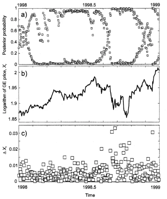
inputs for the filteringformula. The posterior probabilities

$p_{i}(t)$, $\mathrm{i}=2,3$, during

1998-1999

are shown in Fig. $5\mathrm{a}$_, We also show for comparison the $\log$ price $X_{k}$ (panel b) and absolute returns _{$|\Delta_{k}|=|X_{k}-X_{k-1}|$} (panel $\mathrm{c}$). During the

second half of

1998

the market witnessed

a

significant price drop of the

GE

shares (panel

b) associated with increased volatility nicely reflected in the dynamics of $|\Delta_{t}|$ (panel $\mathrm{c}$).

This volatility increase is captured by the posterior probabilities shown in panel $\mathrm{a}$

.

We

found (not shown) that

our

results

are

very stable with respect to the particular choice of the

three-valued

alphabet corresponding to the distribution of Fig. 4 $\mathrm{c},\mathrm{d}$ (say, choosing $\{\hat{a_{\overline{l}}}\}=\{0.05, 0.08, 0.15\}$, etc.).

Remark 7,1 _{The reader could ask why}

_we

_{needthefilteringestimate, ifwe}

_can

_simply

_use

estim ation based only

on

price variations. We do a comparison of that type in Cvitanic, Rozovskii and Zaliapin [4], showing that, in general, the filtering procedure is

more

stable and efficient.

7.2

Intraday data:

IBM

In this section

we

estimate intraday volatility using the data for the IBM company during Nov. 1, 1990 – Jan. 11, 1991. We

use

the dataprior to January 11 to estimate the filter

input parameters, and then apply the filter during January 11 to estimate the volatility. The data set includes 60,328 transactions; almost all of them

occur

between 9:30 AM and 16:30 $\mathrm{P}\mathrm{M}$

.

The transaction time is reported up to

a

second; the

average

time between two consecutive transations (we call this interevent time) is 29 $\mathrm{s}\mathrm{e}\mathrm{c}$. In order to construct the

process $P_{t}$

we

preprocessed the data in the following way. First, all interevent times $T_{i}$

larger than 2 hours

were

replaced with random times $\tilde{T}_{i}$ from the empirical distribution of

interevent times shorter than 2 hours. This way

we

removed the long gaps associated with nights, holidays, and long intraday breaks, and concentrated

on

the price dynamics during the business

hours.

Second, if

several

transactions with different price

were

reported within

one

second (so they

1ave

the

same

time tag),

we

separate themby 0.5 seconds; there

were

6,548 such

cases

(10% of the dataset).

The histogram of the initial alphabet estimates $\tilde{a_{i}}$ (Eqs. (5.8) and (5.10)) is shown in

Fig. 6. While there is no striking multimodal structure, the choice of

$\hat{a_{i}}=\{0.19, 0.33, 0.53, 0.75\}$

seems

reasonable if

one

wants to represent the volatility

as

a

Markov jump

process.

The corresponding estimates of the filter parameters

are:

$\mathrm{A}=\{$

-2.75

0.61 0.88

1.26

$1.32$ -6.08

2.37

2.39

2.91

2.87

-8.55

2.76

5.65

8.86 5.61 -20.12, $[1/\mathrm{h}\mathrm{o}\mathrm{u}\mathrm{r}]$

.

The filtering results

are

illustrated in Fig.

7

where

we

show the estimated volatility and price of IBM shares during the morning hours on January 11, 1991, The

a

posteriori volatility $\hat{v_{t}}$ is obtained in the following way: first,

we find

the expected values

$E(v_{T_{k}}):= \sum_{i=1}^{\overline{M}}p_{t}(T_{k})\hat{a_{i}}$. (7.1)

Then,

we group

the posterior expectations (7.1) into $\overline{M}$

separate values

$\hat{v_{t}}:=\{\hat{a_{\mathrm{i}}}$, $\mathrm{i}=\arg\min_{k=1,\ldots,\overline{M}}|E(v_{1})-\hat{a_{k}}|\}$. (7.2)

The filter detected four volatility bursts. Two of them ($9:35\mathrm{A}\mathrm{M}$ and $11:40\mathrm{A}\mathrm{M}$)

corre-spondto

a

high trading intensity;

one

$(9:50\mathrm{A}\mathrm{M})$ to arapid priceincrease; andone $(10:40\mathrm{A}\mathrm{M})$

to intensive price oscillations (without the net change). We

see

that when price changes

are

mild (in

our

example the price only changes by

fixed

increments of 0.125), the filter effec-tively uses the information on the trading intensity to make a decision about the current volatility.

References

[1] Ait Sahalia, Y. and P. Mykland (2004), Estimating Diffusions with Discretely and Possibly Randomly Spaced Data: A General Theory. Annals

_of

Statistics, 32,

2186-2222.

[2] Barndorff-Nielsen, O.E.)

_Graversen

S.E. and

N. Shephard (2003), Power variation

&

stochastic volatility:

a

review and

some

new

results. Journal

_of

Applied Probability 41A,

133-143.

[3] Cvitanic, J., R. Liptser, and B. Rozovskii (2004), A Filtering Approach to Tracking Volatility from Prices Observed at

Random

Times. Submitted.

[4] Cvitanic, J., Rozovskii, B., Zaliapin, I. (2005), Numerical estimation of volatility values from discretely observed

diffusion

data. Subm itted.

[5] Elliott, R J., Hunter,

W.C.

and Jamieson, B.M.

Drift

and volatility estimation in dis-crete time. Jour,

_of

_{Economic Dynamics}

&

_{Control, 22 (1998),}

_209-218

18

[6] Fouque, J.-P., Papanicolaou, G. and Sircar, R., Derivatives in Financial Markets with Stochastic Volatility, Cambridge University Press, (2000).

[7] Prey, R. and Runggaldier, W. A Nonlinear Filtering Approach to Volatility Estimation with a View Towards High Frequency Data.

International Journal

of

Theoretical

and Applied Finance 4 (2001),

199-210.

[8] Gallant,

A.

R. , andTauchen, G. Reprojecting Partially

Observed

Systems with Appli-cation to Interest Rate Diffusions. Jourmal

_of

the American Statistical

Association

93 (1998), 10-24.

[9] Gourieroux, $\mathrm{C}_{)}$.ARCHModels and Finaicial Applications, Springer (1997).

[10] Jacod, J. and Shiryaev,A. N. Limit Theorems

_for

Stochastic

Processes. Springer-Verlag, NewYork, Heidelberg, Berlin, (1987).

[11] Johannes, M. and N. Poison (2003), MCMC methods for Financial Econometrics,

Preprint.

[12] Kallianpur, G. and Striebel,C, _Stochastic

_differential

equations occurring inthe estima-tion of continuous parameter stochasticprocesses, Teor. Veroyatn. Primen., 14 (1969), 597-622.

[13] Kallianpur, G. and Xiong, J. Assetpricingwith stochasticvolatility. AppL Math. Optim,

43

(2001), pp.

47-62.

[14] Krein, S.G. Linear Equations in Banach Spaces. Birkhauser, Boston, (1982).

[15] Krylov, N.V. and Zatezalo, A. Filtering offinite-state time-non homogeneous Markov

processes,

a

direct approach. Applied Mathematics

a

Optimization 42 (2000), 229-258. [i6] Last, G., Brandt, A. Marked Point Processes on the Real Line: A Dynamic Approach,

Springer-Verlag, NewYork, 1995.

[17] Lions, J.-L. and Magenes, E. Problemes

aux

Limites Non Homogenes et Applications, Dunod, Paris, (1968).

[18] Liptser, $\mathrm{R}.\mathrm{S}$

.

and Shiryaev, $\mathrm{A}.\mathrm{N}.$

. Statistics

of

Random

Processes

$II$

.

Applications,

Springer-Verlag, NewYork, (2000). [19] Liptser, $\mathrm{R}.\mathrm{S}$

.

and Shiryayev, $\mathrm{A}.\mathrm{N}$

.

Theory

of

Martingales. Kluwer Acad. Publ, (1989). [20] Malliavin, P. andMancino, $\mathrm{M}.\mathrm{E}$

.

Fourier

Series

method formeasurementof multivariate

[21] Mikulevicius, R. and Pragarauskas, H. On the Cauchy problem for certain

integro-differential

operators in sobolev and Holder spaces. Lithuanian Mathematical Journal,

32 (1992),

238-263.

[22] Platania, A. and L.C.G. Rogers, Particle Filtering in High Frequency Data, _Preprint,

(2004).

[23] Rogers,

L.C.G.

and Zane,

0.

Designing and estimating models of high-frequency data. Preprint, (1998).

[24] Rozovskii, $\mathrm{B}.\mathrm{L}$. Stochastic Evolution Systems, Linear Theory and Applications to

Non-linear Filtering, Kluwer Acad, Publ., Dordrecht-Boston, (1990).

[25] Runggaldier, $\mathrm{W}.\mathrm{J}$. Estimation via stochastic filtering in financial market models. In :

Mathematics ofFinance (G.Yin and Q.Zhang $\mathrm{e}\mathrm{d}\mathrm{s}.$). Contemporary Mathematics, Vol.

351, pp.309-318, American

Mathematical

Society,

Providence

R.I., (2004) . [26] Wharton Research Data Services available at http:$//\mathrm{w}\mathrm{r}\mathrm{d}\mathrm{s}.\mathrm{w}\mathrm{h}\mathrm{a}\mathrm{r}\mathrm{t}\mathrm{o}\mathrm{n}.\mathrm{u}\mathrm{p}\mathrm{e}\mathrm{n}\mathrm{n}.\mathrm{e}\mathrm{d}\mathrm{u}$

[27] Zaliapin, I., A. Gabrielov, and

V. Keilis-Borok

(2004),

Multiscale

Trend

Analysis.

20

Figure 1; _{Exampleofestimating apriorivalues of filter inputparameters, a)}

_Asset

_log-price

$X_{t}$ (solid line,

left

axis) and its two-valued volatility $v_{t}$ (dashed line, right axis). Param eters of the process are $\{a_{i}\}\approx$

{0.316,

0.632},

$r=0.05$, $\lambda_{12}=\lambda_{21}=1$, $n(a_{1})=n(a_{2})=10^{3}$

,

$p_{i}=1/2$. b)

Process

$P_{t}$ (solid) and its piece-wise linear approximation _{$L_{13}(t)$} (dashed)

corresponding to the

corner

point 1 ofMTA decomposition (see Fig. 2). The approximation is offset by 1 upward for comparison. The global lineartrend of$P_{t}$ isextractedfromboth the processes

for

visual convenience, c) Raw volatility estimate $\tilde{v_{t}}$ (left part) and

distribution

of its distinct values (right part). bue alphabet values

are

depicted by horizontal dashed lines. d) Finalvolatilityestimate $\hat{v_{t}}$

.

hue alphabet values

are

depicted by

horizontal

dashed

Figure 2: MTA spectrum for the

process

illustrated in Fig. la. Shaded lines depict two scaling regions with the transition zone between two

corner

points marked in the figure. The right scaling region has the slope -1,

which

corresponds to a self-affine random walk with

no

persistence. The

left

region deviates from this scaling depicting

a

non-random structure within the

process

$P_{t\}}$. this structure is

due

to the characteristic scales of constant

22

Time,hours $.\sim\underline{u)\simeq\circ}$ $\Xi\varpi$ $.\# y’)0[mathring]_{\circ}$

0.11

0.3

0,5

Estimated volatility _{Estimatedalphabet}

Figure

3:

Filtering synthetic asset price, a) Asset $\log$-price $X_{t}$ (right axis) and true

un-observed volatility $v_{t}$ (left axis). Distinct volatility values

are

depicted by shadows: dark

for $v_{t}=0.5$, light for $v_{t}=0.3$,

none

for $v_{t}=0.1$. b) Aposteriori probabilities $p_{3}(t)$ (dark

squares) and $p_{1}(t)$ (white squares) within the interval shown in a). c) Alphabet estimation.

Histogram of initial volatility estimates $\tilde{a}_{i}$ clearly has

a

three-modal structure. Dashed lines

Figure 4: Estimating volatility for General Electric company during 1962-1998, a) Asset price $S_{t}$ during 1962-2004; market splits

are

depicted by solid

arrows.

The shaded interval

1962-1998

is used for alphabet estimation, b) MTA spectrum for the

process

$P_{t}$ that

corre-sponds to GE $\log$-price dynamics. The transition from a higher slope $(s\approx-2)$ to a lower

one

$(s\simeq-1)$

as

$N$ increases is obvious; it

occu

$\mathrm{r}$ between levels $k=17$ and $k=90$. $\mathrm{c}$),

$\mathrm{d}$)

Histogram ofinitial volatility estimates $\tilde{a}_{i}$ at level

$\mathrm{k}$ $=17$ (panel c) and $k=90$ (panel $\mathrm{d}$).

Th$\mathrm{r}\mathrm{e}\mathrm{e}$-modal structure is prominent within this broad range of levels. Similar results

are

24

$\cross\triangleleft$

1998 1998.5 1999

Time

Figure 5: Estimatingvolatility forGeneral Electriccompany during 1998-1999. a) Posterior probabilities$p_{i}(t)$, $\mathrm{i}=2$ (light squares) and $\mathrm{i}=3$ (dark squares) thatcorrespondtovolatility

values $v_{2}=0.1$

and

$v_{3}=0,15$. b) Dynamics of

the

$\log$-price $X_{t}$. c)

Absolute

returns $|\Delta_{t}|$ of

$U\mathrm{J}\mathrm{C}$ $.\underline{\mathrm{o}}$

co

$Dq\}\Phi \mathrm{O}$ \={o} $\mathrm{D}\mathrm{z}\mathrm{E}\supset\Phi\llcorner$

Figure 6: Bstim ating volatility for IBM

company

during November 1,

1990

– January 10,

1991. Histogram of initial estimates ofvolatility alphabet values $\hat{a_{i}}$, $\mathrm{i}=1$,

$\ldots$ ,$N_{k_{0}}=493$, $k_{0}=300$. $=\mathrm{g}$

.

$\sim$ $\frac{\varpi}{\mathit{0},>}$ $\mathrm{B}\Phi$ $\in\varpi$ $.\overline{\overline{\mathrm{u}^{u_{1}})}}$ $\tilde{\mathrm{f}\mathrm{f}\mathrm{i}}L4\}\dot{q\}‘ \mathfrak{g}}$ $.0^{=}\tilde{\mathrm{S}}$

.

Time

Figure 7: Filtering volatility forIBM company duringJanuary 11,

1991.

a) Posterior volatil-ity vt of Eq. (7.2); b) Price dynamics during the

same

time interval See discussion in Sect.

7.2