On generalizations of the Conway-Gordon theorems (Intelligence of Low-dimensional Topology)

全文

(1)11. On generalizations of the Conway‐Gordon theorems Ryo Nikkuni. Department of Mathematics, Tokyo Woman’s Christian University. 1. Introduction. An embedding f of a finite graph. G. into \mathb {R}^{3} is called a spatial embedding of. image f(G) is called a spatial graph of. G.. A subgraph. \gamma. of. G. G,. and the. homeomorphic to the. circle is called a cycle of G . A cycle of G is also called a k ‐cycle if it contains exactly k vertices, and a Hamiltonian cycle if it contains all of the vertices of G . We denote. the set of all k ‐cycles of G by \Gamma_{k}(G) , and the set of all pairs of two disjoint cycles of G consisting of a k ‐cycle and an l ‐cycle by \Gamma_{k,l}(G) . For a cycle \gamma (resp. a pair of disjoint cycles \lambda ) and a spatial embedding f of G, f(\gamma) (resp. f(\lambda) ) is none other than a knot (resp. a 2‐component link) in f(G) . For a Hamiltonian cycle \gamma of G , we also call f(\gamma)a Hamiltonian knot in f(G) . Let K_{n} be the complete graph on n vertices, that is the graph consisting of n vertices such that each pair of its distinct vertices is connected by exactly one edge. Then let us recall the following Conway‐Gordon theorems, which are very famous theorems in spatial graph theory.. Theorem 1.1 (Conway‐Gordon [6]) (1) For any spatial embedding f of K_{6} , we have. \sum_{\lambda\in\Gam a_{3, }(K_{6}) lk (f(\lambda))\equiv 1. (mod 2) ,. where lk denotes the linking number in \mathbb{R}^{3}.. (2) For any spatial embedding f of K_{7} , we have. \sum_{\gamma\in\Gamma_{7}(K_{7})}a_{2}(f(\gamma) \equiv 1 (mod 2) , where. a_{2}. denotes the second coefficient of the Conway polynomial.. Theorem 1.1 implies that K_{6} is intrinsically linked, that is, every spatial graph of K_{6} contains a nonsplittable 2‐component link, and K_{7} is intrinsically knotted, that is, every spatial graph of K_{7} contains a nontrivial knot. Characterizing all intrinsically linked graphs and intrinsically knotted graphs is an important research theme in spatial graph. theory, see for example [8, §§2‐6]. However, our interest in this article is in another.

(2) 2 direction; it is to generalize the Conway‐Gordon theorems to K_{n} with arbitrary n\geq 6. As far as the author knows, there have been little results about a generalization of the Conway‐Gordon type congruences on K_{n} with n\geq 8 . It is all with the following results.. Theorem 1.2 (1) (Foisy [10], Hirano [12] )^{} For any spatial embedding f of K_{8} , we have. \sum_{\gamma\in\Gamma_{8}(K_{8})}a_{2}(f(\gamma) \equiv 3 (mod 6) (2) (Hirano [12]) Let. n\geq 9. .. be an integer. For any spatial embedding f of K_{n} , we have. \sum_{\gamma\in\Gamma_{n}(K_{n})}a_{2}(f(\gamma) \equiv 0 (mod 2) (3) (Kazakov‐Korablev [17]) Let. n\geq 7. .. be an integer. For any spatial embedding f of. K_{n} , we have. \sum_{p+q=n}\sum_{\lambda\in\Gamma_{p,q}(K_{n})}1k(f(\lambda) \equiv 0 (mod 2). .. On the other hand, let us also recall integral lifts of the Conway‐Gordon theorems for K_{6} and K_{7} proven by the author as follows.. Theorem 1.3 (Nikkuni [21]) (1) For any spatial embedding f of K_{6} , we have. \sum_{\gam a\in\Gam a_{6}(K_{6}) a_{2}(f \gam a) -\sum_{\gam a\in\Gam a_{5}(K_ {6}) a_{2}(f \gam a) =\frac{1}{2}\sum_{\lambda\in\Gam a_{3, }(K_{6}) 1k(f \lambda) ^{2}-\frac{1}{2}. .. (1.1). (2) For any spatial embedding f of K_{7} , we have. \sum_{\gamma\in\Gamma_{7}(K_{7}) a_{2}(f \gamma) -2\sum_{\gamma\in\Gamma_{5} (K_{7}) a_{2}(f \gamma). = \frac{1}{7}(2\sum_{\lambda\in\Gam a_{3,4}(K_{7}) 1k(f \lambda) ^{2}+ 3\sum_{\lambda\in\Gam a_{3, }(K_{7}) 1k(f \lambda) ^{2})-6. .. (1.2). Actually, Theorem 1.1 (1) can be recovered from Theorem 1.3 (1) by multiplying by 2 and taking the mod 2 reduction, and Theorem 1.1 (2) can also be recovered from Theorem 1.3 (2) by multiplying by 7 and taking the mod 2 reduction (note that \sum_{\lambda\in\Gamma_{3,3}(K_{7})}1k(f(\lambda))^{2} is odd as we will see later). Our purposes are to generalize the integral Conway‐Gordon theorems to K_{n} with arbitrary n\geq 6 and to investigate the behavior of the nontrivial Hamiltonian knots and links in a spatial graph of K_{n} . This is a joint work with H. Morishita.. lFor any spatial embedding f of. K_{8} ,. \sum_{\gamma\in\Gamma_{8}(K_{8})}a_{2}(f(\gamma))\equiv 1(mod 2)[12].. Foisy showed that \sum_{\gamma\in\Gamma_{8}(K_{8})}a_{2}(f(\gamma))\equiv 0(mod 3)[10] , and Hirano showed that.

(3) 3 2. Generalizations of the Conway‐Gordon theorems. First, we generalize Theorem 1.3 to K_{n} with arbitrary n\geq 6 as follows.. Theorem 2.1 (Morishita‐Nikkuni [18]) Let. n\geq 6. be an integer. For any spatial embed‐. ding f of K_{n} , we have. \sum_{\gamma\in\Gamma_{n}(K_{n}) a_{2}(f \gamma) -(n-5)!\sum_{\gamma\in\Gamma_ {5}(K_{n}) a_{2}(f \gamma). = \frac{(n-5)!}{2}(\sum_{\lambda\in\Gam a_{3, }(K_{n}) 1k(f \lambda) ^{2}- (\begin{ar ay}{l} n -1 5 \end{ar ay}). Example 2.2 (1) In the case of (2) In the case of. n=7. n=6. in Theorem 2.1, we have (1.1).. in Theorem 2.1, we have. \sum_{\gamma\in\Gamma_{7}(K_{7}) a_{2}(f \gamma) -2\sum_{\gamma\in\Gamma_{5} (K_{7}) a_{2}(f \gamma) =\sum_{\lambda\in\Gamma_{3,3}(K_{7}) 1k(f \lambda) ^{2}- 6 .. (2.1). Though (1.2) and (2.1) are slightly different, since \sum_{\lambda\in\Gamma_{3,4}(K_{7})}1k(f(\lambda))^{2} is twice \sum_{\lambda\in\Gamma_{3,3}(K_{7})}1k(f(\lambda))^{2} (see Example 2.8 (1)), these equations are equivalent. Note that any pair of two disjoint 3‐cycles. \lambda. of K_{n} is not shared by any two different sub‐. graphs of K_{n} isomorphic to K_{6} . Then Theorem 1.1 (1) implies that. \sum_{\lambda\in\Gamma_{3,3}(K_{n})}1k(f(\lambda))^{2}. is greater than or equal to the number of subgraphs of K_{n} isomorphic to K_{6} , that is equal to (\begin{ar y}{l n 6 \end{ar y}) . Thus by Theorem 2.1, we have the following. Corollary 2.3 Let n\geq 6 be an integer. For any spatial embedding f of K_{n} , we have. \sum_{\gamma\in\Gamma_{n}(K_{n}) a_{2}(f \gamma) -(n-5)!\sum_{\gamma\in\Gamma_ {5}(K_{n}) a_{2}(f \gamma) \geq\frac{(n-5)(n-6)(n-1)!}{2\cdot 6!}.. Remark 2.4 Endo‐Otsuki introduced a certain special spatial embedding f_{b} of K_{n}, a canonical book presentation of K_{n}[7] , and Otsuki also showed that f_{b}(K_{n}) contains exactly. (\begin{ar y}{l n 6 \end{ar y}) Hopf links as all of the nonsplittable triangle‐triangle links [22]. Thus the lower bound. of Corollary 2.3 is sharp. Furthermore, every 5‐cycle knot in f_{b}(K_{n}) is trivial. Thus for an integer n\geq 6 , we have. \sum_{\gamma\in\Gamma_{n}(K_{n}) a_{2}(f_{b}(\gamma) =\frac{(n-5)!}{2}( (\begin{ar ay}{l} n 6 \end{ar ay})- (\begin{ar ay}{l} n-1 5 \end{ar ay}) =\frac{(n-5)(n-6)(n-1)!}{2\cdot 6!}. .. (2.2). Moreover, for n\geq 7 , let f and g be two spatial embeddings of K_{n} . Let us consider the difference between \sum_{\gamma\in\Gamma_{n}(K_{n})}a_{2}(f(\gamma)) and \sum_{\gamma\in\Gamma_{n}(K_{n})}a_{2}(g(\gamma)) modulo (n-5)! . By Theorem 2.1, we have. \sum_{\gamma\in\Gamma_{n}(K_{n}) a_{2}(f \gamma) -\sum_{\gamma\in\Gamma_{n}(K_ {n}) a_{2}(g(\gamma). \equiv \frac{(n-5)!}{2}(\sum_{\lambda\in\Gamma_{3, }(K_{n}) 1k(f \lambda) ^{2} -\sum_{\lambda\in\Gamma_{3, }(K_{n}) 1k(g(\lambda) ^{2}) (mod (n-5) !). . (2.3).

(4) 4 \sum_{\lambda\in\Gamma_{3,3}(K_{n})}1k(f(\lambda))^{2}. Note that both. is equal to the parity of. and. \sum_{\lambda\in\Gamma_{3,3}(K_{n})}1k(g(\lambda))^{2}. have the same parity, that. (\begin{ar y}{l n 6 \end{ar y}) . Thus by (2.3), we have. \sum_{\gamma\in\Gamma_{n}(K_{n})}a_{2}(f(\gamma) \equiv\sum_{\gamma\in\Gamma_{n}(K_{n})}a_{2}(g(\gamma) (mod (n-5) !) . This shows that. \sum_{\gamma\in\Gamma_{n}(K_{n})}a_{2}(f(\gamma)). (2.4). does not depend on an embedding f of K_{n} . Now let. us select a canonical book presentation f_{b} of K_{n} as g . Then by (2.2) and (2.4), we have. \sum_{\gamma\in\Gamma_{n}(K_{n}) a_{2}(f \gamma) \equiv\frac{(n-5)!}{2}( (\begin{ar ay}{l} n 6 \end{ar ay})- (\begin{ar ay}{l } n -1 5 \end{ar ay}) ( mod (n-5) !). .. (2.5). (\begin{ar y}{l n 6 \end{ar y}) is odd if and only if n\equiv 6,7(mod 8) , and (\begin{ar ay}{l n-1 5 \end{ar ay}) is odd if and only if n\equiv 0,6(mod 8) . Thus by (2.5), we have the following congruence, that contains Theorem 1.1 (2) and Theorem 1.2 (1) as the cases of n=7,8 and also generalizes Theorem 1.2 (2) remarkably. Then we also note that. Corollary 2.5 Let n\geq 7 be an integer. For any spatial embedding f of K_{n} , we have the following congruence modulo (n-5)! :. \sum_{\gam \inGam _{n}(K_{n})a_{2}(f\gam )\equiv\{begin{ar y}{l -\frac{(n-5)!}{2[Matrix] (n\equiv0(mod8) 0 (n\otequiv0,7(mod8) \frac{(n-5)!}{2[Matrix] (n\equiv7(mod8). \end{ar y}. Next, we also generalize Theorem 1.2 (3) from a viewpoint of the linking numbers of 2‐component “Hamiltonian” links as follows.. Theorem 2.6 (Morishita‐Nikkuni [19]) Let positive integers satisfying n=p+q , where. p,. n\geq 6. be an integer. Let. p. and. q. be two. q\geq 3 . For any spatial embedding f of K_{n},. we have. \sum_{\lambda\inGam a_{p,q}(K_{n})1k(f\lambda)^{2}=\{begin{ar y}{l (n-6)!\sum1k(f\lambda)^{2} (p=q) 2(n-6)!\sum_{\lambda\inGam a_{3,}(K_{n})^{\lambda\inGam a_{3,} 1k(f\lambda)^{2}(K_{n}) (p\neq ). \end{ar y}. In particular, we also have. \sum_{p+q=n}\sum_{\lambda\in\Gamma_{p,q}(K_{n}) 1k(f \lambda) ^{2}=(n-5)!\sum_ {\lambda\in\Gamma_{3,3}(K_{n}) 1k(f \lambda) ^{2}. Theorem 2.6 also implies that for any spatial embedding f of K_{n}(n\geq 6) , the sum of 1k^{2} over all of the Hamiltonian 2‐component links is congruent to 0 modulo (n-5) !.. As we have already seen, \sum_{\lambda\in\Gamma_{3,3}(K_{n})}1k(f(\lambda))^{2} is greater than or equal to by Theorem 2.6, we have the following.. (\begin{ar y}{l n 6 \end{ar y}) .. Thus.

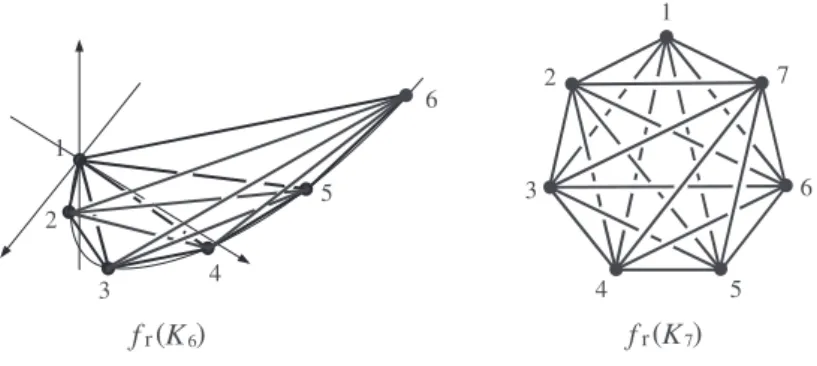
(5) 5 Corollary 2.7 Let n\geq 6 be an integer. Let p and q be two positive integers satisfying n=p+q , where p, q\geq 3 . For any spatial embedding f of K_{n} , we have. In particular,. \sum_{\lambda\in Gam a_{p,q}(K_{n})1k(f\lambda)^{2}\geq\{ begin{ar y}{l \frac{n!}6 (p=q) 2.\frac{n!}6 (p\neq ). \end{ar y} \sum_{p+q=n}\sum_{\lambda\in\Gamma_{p,q}(K_{n}) 1k(f \lambda) ^{2}\geq(n-5) \cdot\frac{n!}{6!}.. Example 2.8 (1) In the case of. n=7. in Corollary 2.7, we have. \sum_{\lambda\in\Gamma_{3,4}(K_{n}) 1k(f \lambda) ^{2}= 2\sum_{\lambda\in\Gamma_{3 }(K_{n}) 1k(f \lambda) ^{2}\geq 14. It has been shown in Fleming‐Mellor [9] that every spatial graph of K_{7} contains at least 14 triangle‐square links with odd linking number.. (2) In the case of. n=8. in Corollary 2.7, we have. \sum_{\lambda\in\Gamma_{3,5}(K_{n}) 1k(f \lambda) ^{2}= 2\sum_{\lambda\in\Gamma_{4,4}(K_{n}) 1k(f \lambda) ^{2}=4\sum_{\lambda\in\Gamma_ {3,3}(K_{n}) 1k(f \lambda) ^{2}\geq 1 2 .. (2.6). It has also been shown in [9] that every spatial graph of K_{8} contains at least 42 nonsplittable triangle‐pentagon links and 35 nonsplittable square‐square links. Based. on (2.6), we expect that every spatial graph of K_{8} contains many more nonsplittable triangle‐pentagon links and square‐square links.. 3. Applications to rectilinear spatial complete graphs. A spatial embedding f_{r} of a simple graph G is said to be rectilinear if for any edge e of G, f_{r}(e) is a straight line segment in \mathb {R}^{3} . We can construct a special rectilinear spatial embedding of K_{n} by taking n vertices of K_{n} on the moment curve (t, t^{2}, t^{3}) in \mathb {R}^{3} and connecting every pair of two distinct vertices by a straight line segment, see Fig. 3.1 for n=6,7^{2} We say such a rectilinear spatial embedding of K_{n} to be standard. A rectilinear spatial graph appears in polymer chemistry as a mathematical model. for chemical compounds (see [1, §7], for example), and the range of rectilinear spatial graph types is much narrower than the general spatial graphs. So we are interested in the behavior of the nontrivial Hamiltonian knots and links in a rectilinear spatial graph of K_{n}. Note that knot and link types appearing as constituent knots and links in a rectilinear spatial graph of K_{n} are limited because they have the stick number \leq n , where the stick number of a link L , denoted by s(L) , is the minimum number of edges in a polygon 2In fact, the standard rectilinear spatiaı graph of. K_{7}. is equivalent to the Conway‐Gordon’s spatial graph of. which contains exactly one trefoil knot as the nontrivial Hamiltonian knots.. K_{7}. in [6].

(6) 6. f_{r}(K_{6}) f_{r}(K_{7}) Figure 3.1: Standard rectilinear spatial embedding f_{r} of K_{n}(n=6,7). representing. L.. We recall the following results on stick numbers (see [1], [20], [2], [5]),. where we denote each of knots and links appearing in the statement by using its label in Rolfsen’s table.. Proposition 3.1 Let. (1) If. L. L. be a link. Then the following statements hold.. is a nontrivial knot, then s(L)\geq 6.. (2) s(L)=6 if and only if. L. is equivalent to 3_{1},0_{1}^{2} or 2_{1}^{2}.. (3) s(L)=7 if and only if. L. is equivalent to 4_{1} or 4_{1}^{2}.. (4) s(L)=8 if and only if. L. is equivalent to 5_{1},5_{2},6_{1},6_{2},6_{3} , the granny knot 3_{1}\# 3_{1},. the square knot 3_{1}\# 3_{1}^{*},8_{19},8_{20} or 5_{1}^{2}.. Proposition 3.1 (1) says that every polygonal knot with five sticks is trivial. Thus for rectilinear spatial graph of K_{n} , by Theorem 2.1 we have the following immediately.. Theorem 3.2 Let n\geq 6 be an integer. For any rectilinear spatial embedding f_{r} of K_{n}, we have. \sum_{\gamma\in\Gamma_{n}(K_{n}) a_{2}(f_{r}(\gamma) =\frac{(n-5)!}{2} ( \sum_{\lambda\in\Gam a_{3, }(K_{n}) lk (f_{r}(\lambda))^{2}- (\begin{ar y}{l n-1 5 \end{ar y}) ). Also note that a 2‐component link with exactly six sticks is either a trivial link or a. Hopf link by Proposition 3.1 (2). Thus for any rectilinear spatial embedding f_{r} of K_{n}, \sum_{\lambda\in\Gamma_{3,3}(K_{n})} lk (f_{r}(\lambda))^{2} is equal to the number of triangle‐triangle Hopf links in f_{r}(K_{n}) . Namely, Theorem 3.2 says that for every rectilinear spatial graph of K_{n}(n\geq 6) , the sum of a_{2} over all of the Hamiltonian knots is determined explicitly in terms of the number of triangle‐triangle Hopf links. In the same way as Corollary 2.3, we can obtain a lower bound of \sum_{\gamma\in\Gamma_{n}(K_{n})}a_{2}(f_{r}(\gamma)) for all rectilinear spatial embeddings f_{r} of K_{n} . On the other hand, since the number of triangle‐triangle Hopf links in a rectilinear spatial graph of K_{6} is strongly limited, we can also obtain an upper bound of \sum_{\gamma\in\Gamma_{n}(K_{n})}a_{2}(f_{r}(\gamma)) . Actually, it is known the following..

(7) 7 Proposition 3.3 (Hughes [15], Huh‐Jeon [14], Nikkuni [21]) Every rectilinear spatial graph of K_{6} contains at most three Hopf links. This implies that \sum_{\lambda\in\Gamma_{3,3}(K_{n})}1k(f_{r}(\lambda))^{2} is less than or equal to 3 (\begin{ar y}{l n 6 \end{ar y}) . Thus by Theorem 3.2, we have the following.. Corollary 3.4 Let n\geq 6 be an integer. For any rectilinear spatial embedding f_{r} of K_{n}, we have. \frac{(n-5)(n-6)(n-1)!}{2\cdot 6!}\leq\sum_{\gamma\in\Gamma_{n}(K_{n})}a_{2} (f_{r}(\gamma) \leq\frac{3(n-2)(n-5)(n-1)!}{2\cdot 6!}. Example 3.5 (1) In the case of. n=6. in Corollary 3.4, we have. 0 \leq\sum_{\gamma\in\Gamma_{6}(K_{6}) a_{2}(f_{r}(\gamma) \leq 1. By Proposition 3.1 (2), f_{r}(\gamma) is either a trivial knot or a trefoil knot. Since a_{2}(3_{1})=1, we have that every rectilinear spatial graph of K_{6} contains at most one trefoil knot,. which was also observed in [14] in combinatorial way. (2) In the case of. n=7 ,. by Corollary 3.4 and Theorem 1.1 (2), we have. 1 \leq\sum_{\gamma\in\Gamma_{7}(K_{7})}a_{2}(f_{r}(\gamma) \leq 15, \sum_{\gamma\in\Gamma_{7}(K_{7})}a_{2}(f_{r}(\gamma) \equiv 1 (mod 2). .. By Proposition 3.1 (2) and (3), if f_{r}(\gamma) is a nontrivial knot then it is either a trefoil. knot or a figure eight knot. Since a_{2}(4_{1})=-1 , we have that every rectilinear spatial graph of K_{7} contains a trefoil knot with 7 sticks, which was originally proven by. Brown [4] and Ramírez Alfonsı’n [24] in combinatorial and computational way. (3) In the case of. n=8 ,. by Corollary 3.4 and Theorem 1.2 (1), we have. 21 \leq\sum_{\gamma\in\Gamma_{8}(K_{8})}a_{2}(f_{r}(\gamma) \leq 189, \sum_{\gamma\in\Gamma_{8}(K_{8})}a_{2}(f_{r}(\gamma) \equiv 3 (mod 6). .. By Proposition 3.1, all of the polygonal knots with 8 sticks are classified completely, and, in addition, only 3_{1},5_{1},5_{2},6_{3},3_{1}\# 3_{1},3_{1}\# 3_{1}^{*},8_{19} and 8_{20} have a_{2} with a positive value. Thus every rectilinear spatial graph of K_{8} contains one of these knots as a Hamiltonian knot. Since the maximum value of a_{2} for them is 5 (a_{2}(8_{19})=5) , we have that the minimum number of nontrivial Hamiltonian knots with a positive value of a_{2} in every rectilinear spatial graph of K_{8} is at least \lceil 21/5\rceil=5 . However this is not yet the sharp lower bound, see Remark 4.2. In Section 4, we will discuss the minimum number of nontrivial Hamiltonian knots in a rectilinear spatial graph of K_{n} with arbitrary n\geq 7. Remark 3.6 The lower bound in Corollary 3.4 is also sharp, actually the standard rec‐ tilinear spatial embedding of K_{n} realizes the lower bound. On the other hand, in the.

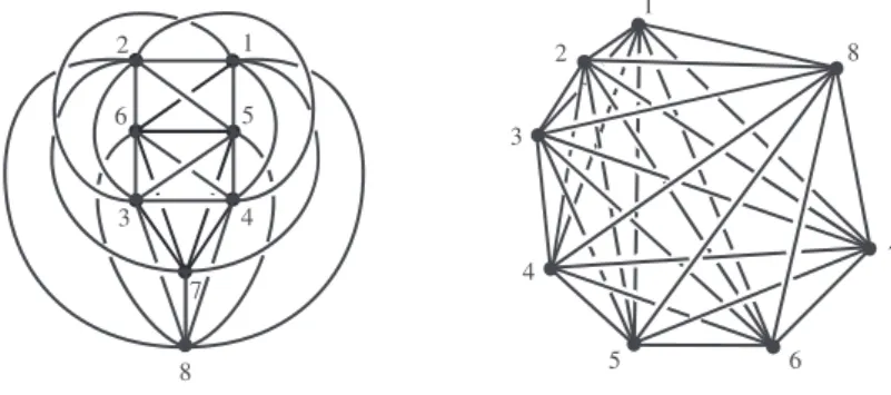
(8) 8 case of. n=7 ,. our upper bound is 15.. However, according to a computer search in. [16] (by using the oriented matroid theory), there seems to be no rectilinear embed‐. \sum_{\gamma\in\Gamma_{7}(K_{7})}a_{2}(f_{r}(\gamma))=13,15 ,. ding f_{r} of K_{7} such that. or equivalently by Theorem 3.2,. \sum_{\lambda\in\Gamma_{3,3}(K_{7})}1k(f_{r}(\gamma))^{2}=19,21 . Thus the author does not expect that the upper bound in Corollary 3.4 is sharp if n\geq 7. Problem 3.7 Determine the sharp upper bound of \sum_{\gamma\in\Gamma_{n}(K_{n})}a_{2}(f_{r}(\gamma)) for all rectilinear spatial embeddings f_{r} of K_{n} for each n\geq 7 , or equivalently by Theorem 3.2, determine the maximum number of triangle‐triangle Hopf links in f_{r}(K_{n}) for each n\geq 7. Example 3.8 Let us consider two spatial embeddings of K_{8} as illustrated in Fig. 3.2.. The left one was given in [3], and the right one is the standard rectilinear spatial em‐ bedding of K_{8} . It is known that, they are not equivalent3 but each of them contains exactly 21 trefoil knots as all of the nontrivial Hamiltonian knots [3], [25]. We did not understand the meaning of this number 21” over ten years. In our current research, we have that for any spatial embedding f of K_{8} , if every 5‐cycle knot in f(K_{8}) is trivial then \sum_{\gamma\in\Gamma_{8}(K_{8})}a_{2}(f(\gamma))\geq 21 . This also implies that if every nontrivial Hamiltonian knot is a trefoil knot, then there must exist at least 21 trefoil knots as Hamiltonian knots.. 8. Figure 3.2: Two spatial embeddings of K_{8}. 4. Further applications. In the rest of this article, we shall mention further two applications. First, let us consider the minimum number of nontrivial Hamiltonian knots in a rectilinear spatial graph of K_{n} . Note that we can obtain an estimate of. a_{2} over Hamiltonian knots in a rectilinear. spatial graph of K_{n} from above as follows. The crossing number of a link L is the minimum number of crossings in a regular diagram of L on the plane, denoted by c(L) . In particular. 3The ıeft spatial graph of. K_{8}. contains a triangle‐pentagon ıink with nonzero even ık (actuaıly [257]\cup[13846] ), but the. right spatial graph of K_{8} does not contain such a triangle‐pentagon link..

(9) 9 for a knot. K,. it has been shown that. c(K) \leq\frac{(s(K)-3)(s(K)-4)}{2}. (4.1). by Calvo [5], and also has been shown that. a_{2}(K) \leq\frac{c(K)^{2} {8}. (4.2). by Polyak‐Viro [23]. By combining (4.1) and (4.2), for a polygonal knot. K. with. \leq n. sticks, we have. a_{2}(K) \leq\lfloor\frac{(n-3)^{2}(n-4)^{2} {32}\rfloor ,. (4.3). where \lfo r\cdot\rflo r denotes the floor function. Then by the lower bound in Corollary 3.4 and (4.3), we have the following estimate of the minimum number of nontrivial Hamiltonian knots in every rectilinear spatial graph of K_{n} from below. Corollary 4.1 Let n\geq 7 be an integer. The minimum number of nontrivial Hamiltonian knots with a positive value of a_{2} in every rectilinear spatial graph of K_{n} is at least. r_{n}= \lceil\frac{(n-5)(n-6)(n-1)!/(2\cdot 6!)}{\lf o r(n-3)^{2}(n-4)^{2} /32\rflo r}\rceil, where \lceil\cdot\rceil denotes the ceiling function. The concrete values of. r_{n}. for 7\leq n\leq 16 are given in the following table.. Remark 4.2 For every spatial embedding f of K_{n} (which does not need to be rectilinear),. Hirano showed that there exist at least three nontrivial Hamiltonian knots with an odd. value of. a_{2}. in f(K_{8})[13] , and Foisy showed that there exist at least (n-1)(n-2)\cdots 9\cdot 8. nontrivial Hamiltonian knots with an odd value of a_{2} in. f(K_{n}). if. n\geq 9[3] .. We see that. is greater than Foisy’s lower bound of the minimum number of nontrivial Hamiltonian knots with an odd value of a_{2} if n=9,10,11 . On the other hand, in the case of n=8 , as r_{n}. we have already seen in Example 3.5 (3), we can obtain an estimate 5” from below better than r_{8} . Moreover, it is known that every rectilinear spatial graph of the complete four‐ partite graph K_{3,3,1,1} contains at least one nontrivial Hamiltonian knot with a positive. value of a_{2} (Hashimoto‐Nikkuni [11]). Since there are 280 subgraphs of K_{8} isomorphic to K_{3,3,1,1} and for any 8‐cycle \gamma of K_{8} there exist 36 subgraphs of K_{8} isomorphic to K_{3,3,1,1} containing \gamma , we have that there are at least \lceil 280/36\rceil=8 nontrivial Hamiltonian knots with a positive value of. a_{2}. in every rectilinear spatial graph of K_{8}.. Problem 4.3 Determine the minimum number of nontrivial Hamiltonian knots (with a positive value of a_{2} ) in every rectilinear spatial graph of K_{n} for each n\geq 8..

(10) 10 Next, we can also obtain the result about the maximum value of Hamiltonian knots in a rectilinear spatial graph of K_{n} as follows.. Theorem 4.4 (Morishita‐Nikkuni [19]) Let. n\geq 6. a_{2}. for all of the. be an integer. For any rectilinear. spatial embedding f_{r} of K_{n} , we have. \max_{\gamma\in\Gamma_{n}(K_{n})}\{a_{2}(f_{r}(\gamma) \}\geq\frac{(n-5)(n-6)} {6!}. Actually, by Corollary 3.4 we have. \max_{\gamma\in\Gamma.(K_{n}) \{a_{2}(f_{r}(\gamma) \}\cdot\#\Gamma_{n}(K_{n}) \geq\sum_{\gamma\in\Gamma_{n}(K_{n}) a_{2}(f_{r}(\gamma) \geq\frac{(n-5)(n-6)(n- 1)!}{2\cdot 6!}, and since \#\Gamma_{n}(K_{n})=(n-1)!/2 , we have the result.4 Theorem 4.4 implies that if. n. is. sufficiently large then every rectilinear spatial graph of K_{n} contains a Hamiltonian knot with arbitrary large value of a_{2} . By Theorem 4.4, we also have the following corollary. Corollary 4.5 Let m be a positive integer. If n>(11+\sqrt{2880m-2879})/2 , then for any rectilinear spatial embedding f_{r} of K_{n} , there exists a Hamiltonian cycle \gamma\in\Gamma_{n}(K_{n}) such that. a_{2}(f_{r}(\gamma))\geq m.. Remark 4.6 It has been shown in Shirai‐Taniyama [26] that (1) For any spatial embedding f of K_{482^{k}} , there exists a cycle. |a_{2}(f(\gamma))|\geq 2^{2k},. (2) Let. m. \gamma. of K_{48\cdot 2^{k}} such that. be a positive integer. If n\geq 96\sqrt{m}, then for any spatial embedding f of K_{n}, \gamma of K_{n} such that |a_{2}(f(\gamma))|\geq m.. there exists a cycle. If we restrict ourselves to rectilinear spatial graphs of K_{n} , Corollary 4.5 is better than Shirai‐Taniyama’s result, see the following table.. For any knot (resp. link) type L , Negami proved in [20] that there exists a positive integer n such that every rectilinear spatial graph of K_{n} contains a knot (resp. link) equivalent to L . The minimum value of such n is called the Ramsey number of L , denoted by R(L) . For a positive integer m , let us define R(m) by the minimum value of n such that every rectilinear spatial graph of K_{n} contains a knot with a_{2}\geq m . For example,. since the standard rectilinear spatial graph of K_{6} (Fig. 3.1) does not contain a trefoil knot, we have R(1)=7 . Note that for a knot type K with a_{2}(K)>0, R(K) is evaluated by R(a_{2}(K)) from below. Problem 4.7 Determine. R(m). for each m\geq 2.. 4Though we can also obtain a simiıar resuıt about the maximum value of 1k^{2} for all of the Hamiltonian links, we omit it..

(11) 11 11. Acknowledgment This work was supported by the Research Institute for Mathematical Sciences, an In‐. ternational Joint Usage/Research Center located in Kyoto University. The author was supported by JSPS KAKENHI Grant Number. JP15K04881. and. JP19K03500.. References. [1] C. C. Adams, The knot book. An elementary introduction to the mathematical the‐ ory of knots. Revised reprint of the 1994 original. American Mathematical Society, Providence, RI, 2004.. [2] C. C. Adams, B. M. Brennan, D. L. Greilsheimer and A. K. Woo, Stick numbers and composition of knots and links, J. Knot Theory Ramifications 6 (1997), 149‐161. [3] P. Blain, G. Bowlin, J. Foisy, J. Hendricks and J. LaCombe, Knotted Hamiltonian cycles in spatial embeddings of complete graphs, New York J. Math. 13 (2007), 11‐16. [4] A. F. Brown, Embeddings of graphs in E^{3} , Ph. D. Dissertation, Kent State University, 1977.. [5] J. A. Calvo, Geometric knot spaces and polygonal isotopy, Knots in Hellas 98, Vol. 2 (Delphi), J. Knot Theory Ramifications 10 (2001), 245‐267. [6] J. H. Conway and C. McA. Gordon, Knots and links in spatial graphs, J. Graph Theory 7 (1983), 445‐453.. [7] T. Endo and T. Otsuki, Notes on spatial representations of graphs, Hokkaido Math. J. 23 (1994), 383‐398. [8] E. Flapan, T. Mattman, B. Mellor, R. Naimi and R. Nikkuni, Recent developments in spatial graph theory, Knots, links, spatial graphs, and algebraic invariants, 81‐102, Contemp. Math., 689, Amer. Math. Soc., Providence, RI, 2017.. [9] T. Fleming and B. Mellor, Counting links in complete graphs, Osaka J. Math. 46 (2009), 173‐201. [10] J. Foisy, Corrigendum to: “Knotted Hamiltonian cycles in spatial embeddings of complete graphs” by P. Blain, G. Bowlin, J. Foisy, J. Hendricks and J. LaCombe,. New York J. Math. 14 (2008), 285‐287. [11] H. Hashimoto and R. Nikkuni, Conway‐Gordon type theorem for the complete four‐ partite graph K_{3,3,1,1} , New York J. Math. 20 (2014), 471‐495.. [12] Y. Hirano, Knotted Hamiltonian cycles in spatial embeddings of complete graphs, Docter Thesis, Niigata University, 2010.. [13] Y. Hirano, Improved lower bound for the number of knotted Hamiltonian cycles in spatial embeddings of complete graphs, J. Knot Theory Ramifications 19 (2010), 705‐708..

(12) 12 [14] Y. Huh and C. Jeon, Knots and links in linear embeddings of K_{6} , J. Korean Math. Soc. 44 (2007), 661‐671. [15] C. Hughes, Linked triangle pairs in a straight edge embedding of K_{6} , Pi Mu Epsilon J. 12 (2006), 213‐218. [16] C.. B. Jeon,. Jung,. W.. S.. G. T.. Jin,. Nam and M.. H. J. Lee, S.. Sim,. S.. J. Park,. H. J.. Huh,. J. W.. Number of knots and links in lin‐. ear K_{7} , slides from the International Workshop on Spatial Graphs (2010), http://www.f.waseda.jp/taniyama/SG2010/ta1ks/19‐7Jeon.pdf. [17] A. A. Kazakov and Ph. G. Korablev, Triviality of the Conway‐Gordon function for spatial complete graphs, J. Math. Sci. (N. Y.)203 (2014), 490‐498.. \omega_{2}. [18] H. Morishita and R. Nikkuni, Generalizations of the Conway‐Gordon theorems and intrinsic knotting on complete graphs,. J. Math. Soc. Japan, to appear.. (arXiv: math. 1807. 02805) [19] H. Morishita and R. Nikkuni, in preparation. [20] S. Negami, Ramsey theorems for knots, links and spatial graphs, Trans. Amer. Math. Soc. 324 (1991), 527‐541. [21] R. Nikkuni, A refinement of the Conway‐Gordon theorems, Topology Appl. 156 (2009), 2782‐2794.. [22] T. Otsuki, Knots and links in certain spatial complete graphs, J. Combin. Theory Ser. B68 (1996), 23‐35. [23] M. Polyak and O. Viro, On the Casson knot invariant, Knots in Hellas 98, Vol. 3 (Delphi), J. Knot Theory Ramifications 10 (2001), 711‐738. [24] J. L. Ramírez Alfonsín, Spatial graphs and oriented matroids: the trefoil, Discrete Comput. Geom. 22 (1999), 149‐158. [25] J. L. Ramírez Alfonsín, Spatial graphs, knots and the cyclic polytope, Beiträge Al‐ gebra Geom. 49 (2008), 301‐314.. [26] M. Shirai and K. Taniyama, A large complete graph in a space contains a link with large link invariant, J. Knot Theory Ramifications 12 (2003), 915‐919. Department of Mathematics, School of Arts and Sciences Tokyo Woman’s Christian University 2‐6‐1 Zempukuji, Suginami‐ku, Tokyo 167‐8585 JAPAN. E‐mail address: [email protected].

(13)