liquids near the glass transition
著者
Tokuyama Michio
journal or
publication title
Physical Review. E
volume
80
number
3
page range
031503
year
2009
URL
http://hdl.handle.net/10097/53645
doi: 10.1103/PhysRevE.80.031503Universality in multicomponent glass-forming liquids near the glass transition
Michio Tokuyama
World Premier International Research Center, Advanced Institute for Materials Research, Tohoku University, Sendai 980-8577, Japan 共Received 25 June 2009; revised manuscript received 7 August 2009; published 11 September 2009兲
The slow dynamics of a single particle in multicomponent glass-forming systems including fragile and strong glasses is studied from a unified point of view. The simulation results on two different systems, bulk glass-forming Cu60Ti20Zr20melt and network-forming SiO2, melt are analyzed by the mean-field theory共MFT兲 recently proposed and are compared with other systems near the glass transition. It is shown that the simulation results for the mean-square displacement are all collapsed into a master curve given by MFT if a long-time self-diffusion coefficient has the same value in each system. It is also shown that each long-time self-diffusion coefficient is described well by a singular function predicted recently from first principles. Thus, we conclude that there exists a simple universal mechanism near the glass transition even among any diversely different glass-forming systems.
DOI:10.1103/PhysRevE.80.031503 PACS number共s兲: 64.70.P⫺, 66.10.C⫺, 61.20.Ja, 83.10.Mj
I. INTRODUCTION
Understanding of the glass transition is one of the pio-neering problems encountered in a wide variety of fields, such as soft-matter science and chemical engineering, which deal with complex systems 关1–4兴. With recent progress in
science and technology the relaxation processes of viscous liquids near the glass transition are extensively studied by experiments and computer simulations 关5,6兴. Several
inter-esting statistical-mechanical theories have been also pro-posed to study this problem, for example, by Götze et al. 关4,7,8兴 and by Medina-Noyola and co-workers 关9–11兴. The
former work is based on a mode-coupling theory 共MCT兲, while the latter is based on a generalized Langevin equation description. Although their approaches are limited to a cal-culation of two-body correlations, their results are quite suc-cessful in some cases. However, it is well known that many-body correlations play an important role near the glass transition and cause a dynamic heterogeneity关12,13兴. Hence,
those correlations are indispensable to discuss the slow re-laxation in complex systems. In general, however, it is diffi-cult to deal with them from first principles. In the present paper, we focus only on the dynamics of a single particle. Instead of calculating those correlations, therefore, we inves-tigate how many-body correlations lead to universal proper-ties in the dynamics of a single particle by just analyzing available data for the mean-square displacement from a uni-fied point of view based on the mean-field theory 共MFT兲 recently proposed 关14,15兴. We do not discuss the dynamics
of the non-Gaussian parameter here since precise data are not available yet.
In this paper, we discuss whether there exists a universal-ity near the glass transition among diversely different glass-forming systems, including fragile glass formers and strong glass formers. In the previous papers关15,16兴, we have shown
that there exists a universality among fragile glass formers. In the present paper, we analyze the simulation results on two different systems, bulk glass-forming Cu60Ti20Zr20 melt
关17兴 and network-forming SiO2 melt 关18兴, from a unified
point of view based on MFT and compare them with the previous results. Thus, we show that the dynamical
proper-ties of the relaxation processes in those systems are also remarkably universal as in fragile systems. The first point is that any dynamical states of the systems are uniquely deter-mined by a long-time self-diffusion coefficient DS
L共or a
uni-versal parameter u兲. The second is that any simulation results for the mean-square displacements in different systems can be described by a single master curve given by MFT at a given value of u. Thus, we show that MFT can describe not only the relaxation processes in fragile glass-forming sys-tems but also those in strong glass-forming syssys-tems. This is also predicted from a first-principles theory recently pro-posed by the present author关19兴.
We begin in Sec. IIby reviewing the theories, which are used in the present paper. In Sec. IIIwe show the universal behavior among different systems from a unified point of view based on the MFT. We conclude in Sec. IV with a summary.
II. THEORIES
We consider three-dimensional multicomponent glass-forming systems, AxByCz¯, which consists of N␣ particles
with mass m␣ and diameter ␣␣ in the total volume V at temperature T, where ␣苸兵A,B,C,...其, N=兺␣N␣, and x + y + z +¯ =100. Let Xi共␣兲共t兲 and Pi共␣兲共t兲 denote the position
vector of ith particle of component ␣ and its momentum at time t.
A. First-principles theory
We first review the first-principles theory recently pro-posed by the present author 关19兴. The particle obeys the
Newton equation d dtPi 共␣兲共t兲 = F i 共␣兲共t兲, 共1兲
where Fi共␣兲共t兲 is a force acting on the ith particle of compo-nent ␣ from the other particles. Equation 共1兲 holds on the
time scale of order tth共=␣␣/vth兲, where vth关=共kBT/m␣兲1/2兴 is
In this paper, we are only interested in the single-particle dynamics near the glass transition, whose space-time scales are much larger than those of microscopic processes. Then, the useful physical quantities to describe the relaxation of a single particle near the glass transition are given by the self-intermediate scattering function
FS共␣兲共q,t兲 = 具exp关iq · 兵Xi共␣兲共t兲 − Xi共␣兲共0兲其兴典 共2兲
and the mean-square displacement
M2共␣兲共t兲 = 具兩Xi共␣兲共t兲 − Xi共␣兲共0兲兩2典, 共3兲
both of which are related through the relation FS共␣兲共q,t兲 ⯝ exp
冋
− q2 6M2 共␣兲共t兲 +q4 2冉
M2共␣兲共t兲 6冊
2 ␣2共␣兲共t兲 + ¯册
, 共4兲 where␣2共t兲 is the non-Gaussian parameter 关20兴.As shown in the previous paper 关19兴, using the
Tokuyama-Mori projection operator method 关21兴, one can
transform Eq. 共1兲 into a time-convolutionless generalized
Langevin equation d dtPi 共␣兲共t兲 = −
冕
0 t 共␣兲共s兲ds P i 共␣兲共t兲 + f i 共␣兲共t兲 共5兲with the memory function
共␣兲共t兲 = 具fi共␣兲共t兲 · fi共␣兲共0兲典
具Pi共␣兲共t兲 · Pi共␣兲共0兲典
, 共6兲
where fi共␣兲共t兲 denotes the fluctuating force and is given by
fi共␣兲共t兲 = Fi共␣兲共t兲 +
冕
0 t 共␣兲共s兲ds P i 共␣兲共t兲. 共7兲 Here, fi共␣兲共t兲 satisfies 具fi共␣兲共t兲 · Pi共␣兲共0兲典 = 具fi共␣兲共t兲典 = 0. 共8兲The use of Eqs.共5兲 and 共8兲 then leads to
具Pi共␣兲共t兲 · Pi共␣兲共0兲典 = exp
冋
−冕
0 t ds冕
0 s d 共␣兲共兲册
具共Pi共␣兲兲2典. 共9兲 Equation共5兲 is a starting equation to discuss the dynamics ofa single particle.
By using Eqs.共3兲 and 共5兲, one can derive the equation for
the mean-square displacement M2共␣兲共t兲 as 关19兴
d dtM2
共␣兲共t兲 = 6D共␣兲共t兲, 共10兲
where D共␣兲共t兲 denotes the time-dependent self-diffusion co-efficient and is given by
D共␣兲共t兲 = 共␣␣v0兲t/tM 1 + t兰0
t共␣兲共s兲ds. 共11兲
Here,v0=共⑀/m␣兲1/2and tM= t0共v0/vth兲2, where⑀is an energy
and t0=␣␣/v0. Let t denote a relaxation time of the
memory function共␣兲共t兲. Then, one finds
M2共␣兲共t兲 ⯝
再
3vth 2t2 for tⰆ t  6DS L t for tⰇ t,冎
共12兲with the long-time self-diffusion coefficient DS
L
= D共␣兲共t = ⬁兲 = ␣␣v0 tM兰0⬁共␣兲共s兲ds
. 共13兲
Thus, there are different time stages, depending on time scales关14兴. In an early stage 共E兲 for tⱕtf, the particle obeys
a ballistic motion. In an intermediate stage 共or stage兲 共兲 for tfⰆtⱕt, it behaves as if it is trapped in a cage which is
mostly formed by neighboring particles. This is the so-called cage effect. On the time scale of order t, the particles can escape their cages and in a late stage共L兲 for tⰇt; they obey a long-time diffusion process with DS
L
.
B. Long-time self-diffusion coefficient
In general, it is difficult to calculate the memory function up to higher order in Fi. However, this is indispensable to
discuss the slow dynamics of a single particle near the glass transition because the many-body correlations play an impor-tant role near the glass transition. As shown in the previous paper关22兴, the long-time self-diffusion coefficient DSLis writ-ten as DS L共兲 ␣␣v0 =␣␣−1
冉
c 共␣兲 冊冉
1 − c共␣兲冊
2 , 共14兲where is a control parameter, such as an inverse tempera-ture 1/T and a volume fraction, andc共␣兲is a singular point
to be determined. The singular part of Eq.共14兲 results from
the long-time correlation effects due to the many-body inter-actions between particles and is in general difficult to calcu-late. Hence, the singular point c is only determined by
fit-ting Eq. 共14兲 with experimental data and simulation results.
As is discussed later, however, there exists a universal rule to determine it.
On the other hand, the coefficient ␣␣ can be calculated analytically. The use of Eqs.共13兲 and 共14兲 then leads to
tM
冕
0 ⬁ 共␣兲共s兲ds = ␣␣冉
c 共␣兲冊冉
1 − c共␣兲冊
−2 , 共15兲As discussed in the previous paper 关22兴, the coefficient␣␣
can be calculated analytically at lower values of for such systems that 共i兲 the intermolecular force is of long range and/or 共ii兲 the number density is nondiluted at lower as
␣␣=⑀␣␣
冏
冉
−U␣␣rep共r兲
r
冊
冏
r=␣␣
, 共16兲
where U␣␣rep共r兲 denotes a repulsive part of the potential U␣␣共r兲. For other systems in which the control parameter is the volume fractionand the intermolecular force is of short range with a linear force range␣␣, an analytical prediction of␣␣is as follows. At lower volume fractions, the two-body repulsive interactions play an important role. In the follow-ing, therefore, we only discuss those interactions. By using Eqs. 共6兲, 共7兲, and 共9兲, one can then write 共␣兲共t兲, up to the
共␣兲共t兲 =具Fi共␣兲共t兲 · Fi共␣兲共0兲典
具共Pi共␣兲兲2典
+ O共Fi
4兲, 共17兲
where 具共Pi共␣兲兲2典=3m␣kBT. It is convenient to introduce the
number densities by nS共␣兲共r兲 =␦„r − Xi共␣兲共0兲…, 共18兲 n共␣兲共r兲 =
兺
i=1 N␣ ␦„r − Xi共␣兲共0兲…. 共19兲Then, the force Fi共␣兲共0兲 can be written as
Fi共␣兲共0兲 =
兺

冕
dr1
冕
dr2F12␣nS共␣兲共r1兲n共兲共r2兲, 共20兲where Fij␣denotes the force acting on the particle i of com-ponent ␣ from the particle j of component. As shown in the previous paper关22兴, the force term Fij␣␣is only needed to
determine␣␣at lower values of. In the following, there-fore, we neglect the forces acting on particle of component␣ from particles of other components. It is convenient to intro-duce the dimensionless variables as
rˆ = r/␣␣, kBT/⑀= 1, nˆ =␣␣3 n,
Fˆ = 共12␣␣ ␣␣/⑀兲F12␣␣, Pˆ共␣兲i = Pi共␣兲/共m␣kBT兲1/2. 共21兲
The average distance between particles is of order␣␣/1/3, while the force range is of order ␣␣. Hence, one can write
rˆ2= rˆ1+ rˆ21⯝ rˆ1+ O共1/3兲, 共22兲
nˆ共␣兲共rˆ2兲 = nˆ共␣兲共rˆ1兲 + rˆ21·ˆ1nˆ共␣兲共rˆ1兲 + O共2/3兲, 共23兲
where rˆ21= rˆ2− rˆ1. Thus, the memory integral can be written
as tM
冕
0 ⬁ ␣共s兲ds = t M 具Pi共␣兲共⬁兲 · Fi共␣兲共0兲典 3m␣kBT ⯝冕
drˆ21Fˆ12␣␣ ⫻冕
drˆ1 具Pˆi共␣兲共⬁兲nˆS共␣兲共rˆ1兲rˆ21·ˆ1nˆ共␣兲共rˆ1兲典 3 共24兲 =冋
−冕
1 ⬁ drˆ21rˆ213 Uˆ␣␣rep共rˆ21兲 rˆ21册
⫻冋
冕
drˆ1 4 3 具nˆ 共␣兲共rˆ 1兲Pˆi共␣兲共⬁兲 · ˆ1nˆS共␣兲共rˆ1兲典册
. 共25兲 The second part of Eq.共25兲 is of order 1 and corresponds tothe singular part of Eq.共15兲. Hence, we thus find
␣␣=
冕
1 ⬁ drˆ rˆ3冉
−U ˆ ␣␣ rep共rˆ兲 rˆ冊
. 共26兲As a simple example, we take U␣␣共r兲=kBT共␣␣/r兲n␣␣. Then,
we obtain
␣␣=
n␣␣
n␣␣− d, 共27兲
where d = 3 here. As n␣␣ increases, ␣␣ decreases to 1. In fact, for hard spheres where U␣␣共r兲 is given by the step func-tion, we find␣␣= 1.
In order to test Eq.共27兲, we analyze the simulation results
from Refs. 关23–27兴 for the long-time self-diffusion
coeffi-cient DSL on the polydisperse systems of soft spheres and quasihard spheres with ␦% size polydispersity, where the potential is given by U共r兲=kBT共/r兲n. For comparison, the
hard-sphere systems with ␦% size polydispersity are also considered. In Fig. 1, DS
L/
v0 versus the volume fraction 共=3N/6V兲 is plotted for different values of n. It is thus
shown that for soft spheres with n = 8, ␣␣ is given by Eq. 共16兲, while for quasihard spheres with nⱖ36 it is given by
Eq. 共27兲. On the other hand, for such systems with 9ⱕn
⬍36 that they are neither soft spheres nor hard spheres,␣␣
is only determined by fitting since there is no theory for it. The coefficient␣␣and the singular volume fraction care
listed in Table I. In order to check the consistency with Eq.
FIG. 1. 共Color online兲 A logarithmic plot of DSL/v0versus for different n. The filled squares indicate the simulation results from Ref. 关23兴 and the filled circles indicate the MCT solutions from Ref.关23兴 at n=36 and␦= 10%. The other symbols indicate the simulation results:共䊐兲 n=36 共␦= 10%兲 and 共⫻兲 n=36 共15%兲 from Ref.关24兴, 共䉺兲 n=8, 共〫兲 n=12, 共䉭兲 n=18, 共䊊兲 n=36, and 共+兲 n = 144 at ␦= 0% from Ref.关25兴, and 共䉯兲 hard spheres at ␦= 6% from Ref.关27兴 and 共䉮兲 hard spheres at␦= 15% from Ref.关26兴. The solid and the dashed lines indicate the mean-field singular function given by Eq.共14兲, where and care listed in TableI.
共14兲 more clearly, we also show a log-log plot of DS L/
v0
versus 共c/兲共1−/c兲2 in Fig.2. Thus, all the simulation
results are shown to be well described by Eq. 共14兲 within
errors. Finally, we note here that the simulation results on the polydisperse system with␦= 10 and the corresponding solu-tions of the MCT关23兴 are also well described by Eq. 共14兲. In
both cases␣␣has the same value as 36/33共⯝1.091兲, while the singular pointcis different from each other because the
only two-body correlations are taken into account for MCT but the many-body correlations are done for the simulations. Finally, we note that the simulation results deviate from the mean-field line given by Eq.共14兲 at higher volume fractions.
As is discussed later, this deviation always occurs around the same value of DS
L/
␣␣v0even in different systems.
C. Mean-field theory
Here, we briefly summarize the MFT of the glass transi-tion for molecular systems recently proposed by the present
author关14,15,28兴. The mean-field theory consists of two
es-sential points: 共i兲 the field equations for the mean-square displacement and 共ii兲 the singular long-time self-diffusion coefficients.
Mean-field equations
The mean-square displacement M2共␣兲共t兲 for molecular sys-tems is described by a nonlinear equation 关14兴
d dtM2 共␣兲共t兲 = 6D S L共兲 + 6关v 0 2t − D S L共兲兴e−M2共␣兲共t兲/ᐉ共兲2 , 共28兲 where the mean-free pathᐉ共兲 is a length in which a particle can move freely without any interactions between particles. Although it is originally related to the static structure factor S共q兲 关28兴, it is determined by a fitting with data here.
Equa-tion 共28兲 can be solve to give a formal solution
M2共␣兲共t兲 = 2dDS L t +ᐉ2ln
冋
e−2dt/t+1 6冉
t tf冊
2 ⫻再
1 −冉
1 +2dt t冊
e −2dt/t冎
册
, 共29兲 where t共=ᐉ2/DSL兲 denotes a time for a particle to diffuse
over a distance of order ᐉ with the diffusion coefficient DS L
and is identical to the so-called -relaxation time. Here, tf共
=ᐉ/v0兲 is a mean-free time, within which each particle can
move freely without any interactions between particles. As shown in the previous paper 关15兴, the mean-free path ᐉ is
uniquely determined by DSL/共␣␣v0兲. Hence, solution 共29兲
suggests that the dynamics is described by only one param-eter DS
L/共
␣␣v0兲 if the length and the time are scaled by␣␣
and t0, respectively.
Solution 共29兲 also shows the asymptotic forms given by
Eq. 共12兲. As shown in the previous paper 关14兴, for ⱖs
there exists a new time stage, the so-called-relaxation stage 共兲 for tfⰆtⱕt, where sis a value at which a new time
appears. In fact, one can find one more time scale, the caging time t␥, as follows. First, one can obtain the following asymptotic solutions from Eq. 共29兲:
TABLE I.␣␣andc. Method n ␣␣ c ␦ 共%兲 Ref. MD 8 8关Eq. 共16兲兴 1.245 0 关25兴 MD 12 4共fitting兲 0.822 0 关25兴 MD 18 3共fitting兲 0.6885 0 关25兴 MD 144 144/141关Eq. 共22兲兴 0.5598 0 关25兴 MD 36 36/33关Eq. 共22兲兴 0.593 10 关24兴 MD 36 36/33关Eq. 共22兲兴 0.593 15 关24兴 MD 36 36/33关Eq. 共22兲兴 0.593 10 关23兴 MCT 36 36/33关Eq. 共22兲兴 0.5136 10 关23兴 MD ⬁ 1关Eq. 共22兲兴 0.583 6 关27兴 MD ⬁ 1关Eq. 共22兲兴 0.5908 15 关26兴
FIG. 2. 共Color online兲 A log-log plot of DSL/v0 versus 共c/兲共1−/c兲2 for different n. The details are the same as in
M2共t兲 ⯝
再
ᐉ2ln关1 + 共t/t f兲2兴 for t ⱕ tf 6DS L t for tⱖ tL,冎
共30兲 where tL共=␣␣2 /DSL兲 is a long-diffusion time. We now
intro-duce the logarithmic derivatives by
1共t,兲 = log tlog兩M2共t兲 − ᐉ 2ln关1 + 共t/t f兲2兴兩, 共31兲 2共t,兲 = log t1共t兲. 共32兲
Then, 2共t兲=0 gives two time roots, t␥and t, which reveal two fairly flat regions for ⬎s 关14兴:
1共t兲 =
再
b␥ for t = t␥
b for t = t,
冎
共33兲where b␥= band t␥= t at=s, and b⬎b␥and t⬎t␥for
⬎s. On a time scale of order t␥, each particle behaves as
if it is trapped in a cage, which is mostly formed by neigh-boring particles. This is the so-called cage effect. Hence, the  stage is separated into two stages: a fast stage共f兲 for
tfⰆtⰆt and a slow  stage 共s兲 for t␥ⰆtⰆtL. On a time
scale of order t, the particles can escape their cages, and on a time scale of order tLthey finally obey a long-time
diffu-sion process. By expanding M2共␣兲共t兲 in powers of ln共t/t␥兲 or ln共t/t兲 on each stage, one can then find the following asymptotic forms: M2共␣兲共t兲 ⯝
冦
ᐉ2再
ln冋
1 +冉
t␥ tf冊
2册
+ 2 ln冉
t t␥冊
+ B␥冉
t t␥冊
b␥冎
for 关f兴, ᐉ2再
ln冋
1 +冉
t tf冊
2册
+ B冉
t t冊
b冎
for 关s兴,冧
共34兲where B␣ is a positive constant and b␥and b are time ex-ponents to be determined. We mention here that in stage共f兲
the logarithmic growth dominates the dynamics for all sys-tems since B␥Ⰶ1, while in stage 共s兲 the power-law growth
dominates the dynamics. As increases, both exponents b␥ and b decrease and become constant as b␥= 1.0 and b = 1.3301. We should note here that, since bⱖ1, the power-law behavior in stage 共s兲 is superdiffusion type and is
dif-ferent from that of von Schweidler type.
The single-particle dynamics is determined by only one parameter DS
L/共
␣␣v0兲. Hence, it is convenient to introduce a
parameter u by
u = log10共␣␣v0/DS
L兲. 共35兲
As shown in the previous paper 关15兴, as is increased, the
supercooled state and the glassy state appear at  共u兲 and g 共ug兲, respectively, where g⬎⬎s 共ug⬎u⬎us兲.
Analyses of various data show that u⯝2.6, ug⯝5.1, and
us⯝1.06 共Table II兲. As increases, the time exponents b␥
and b decrease. In the supercooled region 关S兴 for uⱕu ⬍ug, the exponent breduces to 1.3301, while the exponent
b␥reduces to 1 in the glass region关G兴 for uⱖug. We should
also mention here from the detailed analyses that, as u in-creases, the long-time self-diffusion coefficients obtained by the simulations and the experiments start to deviate from Eq. 共14兲 at u=ux共⯝3.04兲, while their mean-square displacements
also show a deviation from Eq.共29兲 for u⬎uxbut only in the
stage. This concurrence may not be a coincidence because the systems are considered not to be in equilibrium for u ⬎ux.
III. UNIVERSALITIES NEAR THE GLASS TRANSITION
In this section, we analyze the mean-square displacements obtained in two different systems, Cu60Ti20Zr20 and SiO2,
from a unified point of view based on MFT and explore universal behavior near the glass transition. Both systems satisfy the conditions that 共i兲 the intermolecular force is of long range and/or 共ii兲 the number density is nondiluted at lower. Hence, ␣␣ is calculated from Eq.共16兲.
TABLE II. Universal parameter u.
us u ux ug
1.06 2.60 3.04 5.10
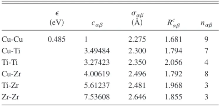
TABLE III. SW potential parameters for Cu60Ti20Zr20from Ref. 关30兴. ⑀ 共eV兲 c␣ ␣ 共Å兲 R␣c n␣ Cu-Cu 0.485 1 2.275 1.681 9 Cu-Ti 3.49484 2.300 1.794 7 Ti-Ti 3.27423 2.350 2.056 4 Cu-Zr 4.00619 2.496 1.792 8 Ti-Zr 5.61237 2.481 1.968 3 Zr-Zr 7.53608 2.646 1.855 3
A. Cu60Ti20Zr20
First, we analyze the simulation results for self-diffusion of Cu in Cu60Ti20Zr20 melt 关17兴, where =1/T. The
molecular-dynamics 共MD兲 simulations are performed at mCu= mTi= mZr by the so-called NPT method by using the
following Stillinger-Weber potential共SW兲 关29兴:
U␣共r兲 =
冦
c␣⑀冋
冉
␣ r冊
n␣ − 1册
exp冋
冉
r ␣− R␣ c冊
−1册
for r⬍ R␣c ␣ 0 for r⬎ R␣c ␣,冧
共36兲where the potential parameters are listed in Table III. Here, the total number of particles is N = 4000. The simulation is done at 1 atm. Length, time, and temperature are scaled by CuCu,CuCu共mCu/⑀兲1/2, and⑀/kB, respectively.
In Fig. 3, the mean-square displacement M2共t兲 for Cu is plotted versus time t/t0for different temperatures. The
mean-field equation given by Eq. 共29兲 agrees with the simulation
results well, except for lower temperatures T⬍Tx. Here, two
adjustable parametersᐉ and DS L
are used to fit Eq.共29兲 with
the simulation results. For T⬍Tx共or u⬎ux兲, the simulation
results deviate upward from the theoretical results only in stage. Hence, those simulation results are considered not to reach an equilibrium state yet. As mentioned before, such a deviation always occurs at u⬎ux. In Fig. 4, the long-time
self-diffusion coefficient DS L
is plotted versus inverse tem-perature. From Eq.共16兲, the coefficientCuCuis calculated as
CuCu= 9 关22兴. The inverse singular temperature is obtained
by fitting Eq. 共14兲 with the simulation results as 1/Tc
⯝5.92. Thus, Eq. 共14兲 can describe the simulation results
well, except for lower temperatures T⬍Tx 共or u⬎ux兲. We
note here that those simulation results also show a deviation from Eq.共14兲 for u⬎ux. Hence, the simulation results do not
reach an equilibrium state yet for u⬎ux. The characteristic
temperatures are listed in Table IV.
B. SiO2
Next, we analyze the simulation results for self-diffusion of O in SiO2 melt 关18兴, where =1/T. The
molecular-dynamics simulations are performed by the so-called NVT method by using the following potential given by Nakano et al. 关31兴: U =
兺
␣⬍U␣ 共2兲+兺
␣,⬍␥U␣␥ 共3兲 共37兲with the two-body potential U␣共2兲共r兲 =⑀
冉
a␣␣+ a r冊
n␣ +Z␣Z r e −r/A0−a␣Z 2+ a Z␣2 2r4 e −r/A1 共38兲 and the three-body potentialU␣␥共3兲 = B␣exp
冋
1 r␣− A2 + 1 r␣␥− A2册
冉
r␣· r␣␥ r␣r␣␥ − cos¯␣冊
2 共A2− r␣兲共A2− r␣␥兲, 共39兲where 共x兲 is a step function, A0= 4.43 共Å兲, A1= 2.5 共Å兲, and A2= 5.5 共Å兲. The potential parameters are listed in Table
V. Here, the total number of particles is N = 5184 and the system size is 42.8 Å. Length, time, and temperature are scaled by OO共=2aOO兲, OO/v0, and ⑀/kB, respectively,
where mO= 2.66⫻10−26 共kg兲 and OOv0= 7.52
⫻10−7 共m2/s兲.
TABLE IV. Characteristic temperatures for Cu.
Ts T Tx Tc Tg
0.399 0.196 0.185 0.169 0.146
2247共K兲 1104共K兲 1042共K兲 952共K兲 822共K兲 FIG. 3.共Color online兲 A log-log plot of M2共Cu兲共t兲 versus time t/t0
for different temperatures, T = 0.315, 0.3, 0.27, 0.23, 0.2, 0.182, 0.167, 0.154, and 0.143共from left to right兲. The filled circles indi-cate the simulation results for Cu from Ref. 关17兴. The solid lines indicate the mean-field master curve given by Eq.共29兲.
In Fig. 5, the mean-square displacement M2共t兲 for O is
plotted versus time t/t0for different temperatures. The mean-field equation agrees with the simulation results well, except for lower temperatures T⬍Tx共or u⬎ux兲. In Fig.6, the
long-time self-diffusion coefficient DS L
is plotted versus inverse temperature. From Eq.共16兲, the coefficientOOis calculated
as OO= 15.31关22兴. The inverse singular temperature is
ob-tained by fitting Eq. 共14兲 with the simulation results as
1/Tc⯝6.0. Thus, Eq. 共14兲 can describe the simulation results
well, except for lower temperatures T⬍Tx 共or u⬎ux兲. This
situation is the same as that discussed in Cu. The character-istic temperatures are listed in TableVI.
In order to show whether Eq. 共14兲 holds for the other
network glass formers, we analyze the data given by Hem-mati and Angell for different model potentials of SiO2 关32兴.
As shown in the previous paper 关22兴, the coefficient OO
should be the same as that obtained by using Eq. 共37兲, even
though the model potentials are different. Hence, we take OO= 15.31 andOOv0= 7.52⫻10−7 共m2/s兲 to analyze seven
different data discussed in Ref. 关32兴. In Fig. 7, we show a
logarithmic plot of the oxygen self-diffusion coefficient DS
L共O兲
versus the reduced temperature Tc/T. The inverse
sin-gular temperatures are obtained by fitting Eq. 共14兲 with the
simulation results and are listed in Table VII. For compari-son, the simulation results obtained by using Eq. 共37兲 are
also shown in Fig.7. In Fig.8, a log-log plot of DS L共O兲
versus 共T/Tc兲共1−Tc/T兲2 is also shown to check consistency with
Eq. 共14兲. All simulation results obtained by using different
potentials are well described by a single master curve given by Eq. 共14兲 up to ux. This is reasonable because most of
those potentials have been made, so that their static structure factors describe realistic structural properties of SiO2. Here, we note that the potential difference appears only in the sin-gular temperature.
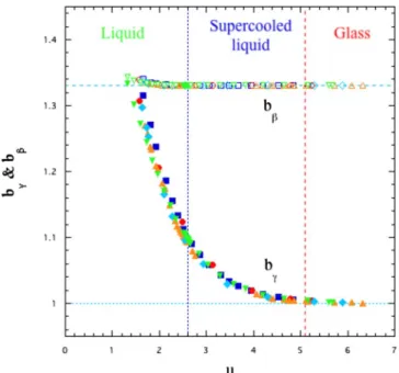
C. Exponents band b␥
We now discuss the exponents b␥ and b obtained for Cu60Ti20Zr20and SiO2. They are calculated numerically from
Eqs.共31兲 and 共32兲 by using fitting values of ᐉ and DS L
. In Fig.
TABLE V. Potential parameters for SiO2. ⑀ 共eV兲 a␣ 共Å兲 Z␣共e兲 a␣ 共Å3兲 n ␣ B␣ 共eV兲 ¯␣ O-O 1.592 1.2 1.76 2.4 7 Si-Si 1.592 0.47 −0.88 0.00 11 O-Si 1.592 9 O-Si-O 4.993 109.47 Si-O-Si 19.972 141.00
FIG. 4. 共Color online兲 A logarithmic plot of DSL共Cu兲versus 1/T. The filled circles indicate the simulation results from Ref.关17兴. The solid lines indicate the mean-field singular function given by Eq. 共14兲, whereCuCu= 9 and 1/Tc= 5.92. A log-log plot of DS
L共Cu兲 ver-sus 共T/Tc兲共1−Tc/T兲2is given in the inset, where the dotted line indicates −ux.
FIG. 5. 共Color online兲 A log-log plot of M2共O兲共t兲 versus time t/t0 for different temperatures, T = 0.2706, 0.2273, 0.2057, 0.1813, 0.1678, 0.1516, 0.1407, and 0.1353共from left to right兲. The filled circles indicate the simulation results for O from Ref. 关18兴. The solid lines indicate the mean-field master curve given by Eq.共29兲.
9, they are plotted versus u. As typical examples of fragile systems, the simulation results for the hard-sphere fluids with 15% size polydispersity关26兴 and 6% size polydispersity 关27兴
and the Lennard-Jones 共LJ兲 binary mixtures 关33兴 are also
plotted for comparison. As u increases, b and b␥ decrease and reduce to each the constant 1.3301 at a supercooled point u and 1.0 at a glass point ug, respectively. Although the
systems are completely different from each other, all their exponents coincide with each other within error. This univer-sality is already seen in fragile systems关15兴.
D. Mean-free path艎
We next discuss the mean-free path ᐉ obtained for Cu60Ti20Zr20 and SiO2. In Fig.10, it is plotted versus u for
different systems. For comparison, the simulation results for the hard-sphere fluids and the Lennard-Jones binary mixtures are also shown. The lengthsᐉ of O and Cu do not agree with other fragile systems. But if one scales ᐉ of O and Cu by 1.8OOand 1.5CuCu, respectively, then they agree with
oth-ers. Those scaled fittings are needed because ␣␣ is not a diameter of O or Cu but just a technical number to make the length scale dimensionless. We note that ᐉ of Cu does not agree with others in a liquid state. This would be because the
simulations on Cu have been done by the NPT method, while the other simulations have been done by the NVT method.
E. Characteristic times tand t␥
We also discuss the characteristic times tand t␥obtained for Cu60Ti20Zr20and SiO2. In Fig.11, they are plotted versus
u. For comparison, the simulation results for the hard-sphere fluids and the Lennard-Jones binary mixtures are also shown. The u dependence of those times are similar to each other, where the results for O and Cu are also scaled by the times 1.8OO/v0 and 1.5CuCu/v0, respectively, as in Fig.10.
F. Mapping
In this section, we discuss a dynamical mapping from one system to another at a given value of DS
L关
16兴. We consider
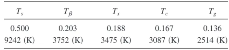
TABLE VI. Characteristic temperatures for O.
Ts T Tx Tc Tg
0.500 0.203 0.188 0.167 0.136
9242共K兲 3752共K兲 3475共K兲 3087共K兲 2514共K兲
TABLE VII. Singular temperatures for different models.
Model 1000/T 共K−1兲 Symbol Ref. Modified-Matsui 0.350 䊊 关32兴 Tsuneyuki 0.305 䉯 关32兴 BKS 0.285 〫 关32兴 Horbach共BKS兲 0.267 䊐 关32兴 Poole 0.200 䉮 关32兴 TRIM 0.1976 ⫻ 关32兴 Kubicki 0.1905 + 关32兴 Nakano 0.324 䉺 关31兴
FIG. 6. 共Color online兲 A logarithmic plot of DSL共O兲versus 1/T. The filled circles indicate the simulation results from Ref.关18兴. The solid lines indicate the mean-field singular function given by Eq. 共14兲, whereOO= 15.31 and 1/Tc= 6.0. A log-log plot of DSL共O兲 ver-sus 共T/Tc兲共1−Tc/T兲2is given in the inset, where the dotted line
indicates −ux.
FIG. 7. 共Color online兲 A logarithmic plot of DSL共O兲versus Tc/T for different models of SiO2. The symbols indicate the simulation results from Ref. 关32兴, except that with the symbol 共䉺兲 is from 关18兴. The solid lines indicate the mean-field singular function given by Eq. 共14兲, where OO= 15.31 and OOv0= 7.52⫻10−7 关m2/s兴. The singular temperatures are listed in TableVII.
the following three cases. The first is a mapping from Cu to the hard-sphere fluid with 6% size polydispersity共HSF6%兲. In Fig.12, the mean-square displacement M2共t兲 is compared
at two different values of DSL; in a liquid state 关L兴 at DS
L/共
v0兲⯝0.05, where = 0.45 for the hard-sphere fluid and T = 0.27 for Cu, and in a supercooled liquid state关S兴 at DS
L/共
v0兲⯝0.0017, where = 0.56 and T = 0.182. At each
value the simulation results are collapsed on the mean-field master curve. Here, we note that in a supercooled state the simulation results for Cu deviate from the mean-field theory because they do not reach an equilibrium state yet.
FIG. 8. 共Color online兲 A log-log plot of DSL共O兲versus 共T/Tc兲共1 − Tc/T兲2. The dashed line indicates −ux. The details are the same as
in Fig.7.
FIG. 9. 共Color online兲 A plot of b␥and bversus u for different systems. The open symbols indicate the exponent band the filled symbols indicate b␥;共䊊兲 Cu, 共䊐兲 O, 共〫兲 hard-sphere fluids with 15 % size polydispersity from Ref.关26兴, 共䉭兲 hard-sphere fluids with 6 % size polydispersity from Ref. 关27兴, and 共䉮兲 LJ from Ref. 关33兴. The horizontal dotted line indicates b␥= 1.0 and the horizontal dashed line indicates b= 1.33014. The vertical dotted line indicates uand the vertical dashed line indicates ug.
FIG. 10. 共Color online兲 A plot of ᐉ/ versus u for different systems. The open squares and circles indicate the original results for O and Cu, respectively, and the filled squares and circles the scaled ones. The details are the same as in Fig.9.
FIG. 11. 共Color online兲 A plot of t␥and tversus u for different systems. The open symbols indicate the time tand the filled sym-bols indicate t␥. The details are the same as in Fig.9.
The second is a mapping from O to the hard-sphere fluid with 15% size polydispersity 共HSF15%兲. In Fig. 13, the mean-square displacement M2共t兲 is compared at two differ-ent values of DS
L
: in a liquid state关L兴 at DS L/共
v0兲⯝0.0053,
where= 0.55 for the hard-sphere fluid and T = 0.2273 for O, and in a supercooled liquid state关S兴 at DSL/共v0兲⯝0.00036, where= 0.58 and T = 0.1678. At the same value of DS
L
, the simulation results are collapsed on the corresponding mean-field master curves given by Eq.共29兲.
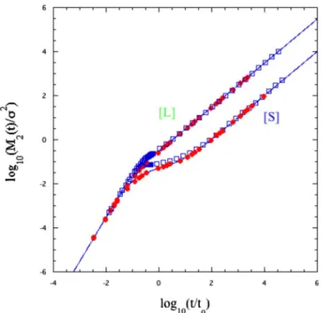
The last is a mapping from O and Cu to the LJ binary mixtures. In Fig.14, the mean-square displacement M2共t兲 is
compared at two different values of DS L
: in a liquid state关L兴 at DS
L/共
v0兲⯝0.01, where T=1.0 for LJ and T=0.23 for Cu,
and in a supercooled liquid state 关S兴 at DS L/共
v0兲⯝0.002, where T = 0.769 for LJ and T = 0.2165 for O. At the same value of DS
L
all the simulation results on fragile and strong glass formers are collapsed on the mean-field master curve given by Eq. 共29兲. Hence, the dynamical behavior in
differ-ent systems is iddiffer-entical to each other if DS L
is the same. This universality is also true even for stronger glass formers, al-though this was discussed only in fragile glass formers in the previous paper关16兴.
G. Long-time self-diffusion coefficient
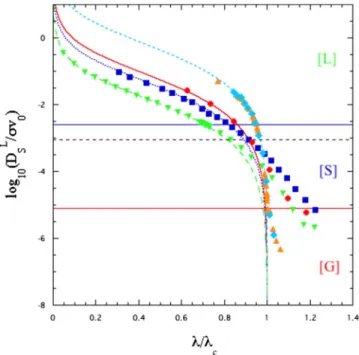
Finally, we discuss the universality among the long-time self-diffusion coefficients for diversely different glass-forming systems. In Fig. 15, DSL is plotted versus /c for
different systems. All simulation results are described by the master curve given by Eq.共14兲 well, except for higher values
FIG. 12. 共Color online兲 A log-log plot of M2共t兲/2versus t/t 0 for two different systems: HSF6% and Cu60Ti20Zr20. The filled circles indicate the simulation results for hard spheres with 6% size polydispersity at关L兴 =0.45 and 关S兴 0.56 from Ref. 关27兴 and the open squares for Cu at关L兴 T=0.27 and 关S兴 0.182 from Ref. 关17兴. The solid lines indicate the mean-field master curve given by Eq. 共29兲.
FIG. 13. 共Color online兲 A log-log plot of M2共t兲/2versus t/t0 for two different systems: HSF15% and SiO2. The filled circles indicate the simulation results for hard spheres with 15% size poly-dispersity at关L兴=0.55 and 关S兴 0.58 from Ref. 关26兴 and the open squares for O at关L兴 T=0.2273 and 关S兴 0.1678 from Ref. 关18兴. The solid lines indicate the mean-field master curve given by Eq.共29兲.
FIG. 14. 共Color online兲 A log-log plot of M2共t兲/2versus t/t 0 for three different systems: LJ, Cu60Ti20Zr20, and SiO2. The filled circles indicate the simulation results for LJ at 关L兴 T=1.0 and 关S兴 0.769 from Ref.关33兴, the open circles for Cu at 关L兴 T=0.23 from Ref.关17兴, and the open squares for O at 关S兴 T=0.2165 from Ref. 关18兴. The solid lines indicate the mean-field master curve given by Eq.共29兲.
/x⬎1 共or u⬎ux兲, where the systems do not reach an
equi-librium state yet. In order to check consistency with Eq.共14兲
more clearly, we also show a log-log plot of DS L/
v0versus 共c/兲共1−/c兲2 in Fig.16. Thus, all the simulation results
are shown to be described by Eq. 共14兲 well up to x over
which the deviation from Eq.共14兲 starts to occur. Hence, this
suggests that the /c dependence of DS L
in any systems should be the same for/xⱕ1 关22兴. This is clearly seen in
Fig.17, where DSL is plotted versus/cfor different
sys-tems. When /x⬎1 共or u⬎ux兲,DS L
obeys a nonsingular function and its value is larger for stronger glasses. For /c⬎1, however, the systems are usually out of
equilib-rium. In order to calculate such a nonsingular function, there-fore, one has to discuss the nonequilibrium relaxation pro-cesses separately from the equilibrium formulation discussed here.
IV. SUMMARY
In this paper, we have analyzed two different glass-forming systems, bulk glass-glass-forming Cu60Ti20Zr20 melt and
network-forming SiO2melt, from a unified viewpoint based on the mean-field theory. We have first shown that the both simulation results for the mean-square displacement M2共t兲
are well described by the mean-field master curve given by Eq. 共29兲, except for lower temperatures T⬍Tx 共or u⬎ux兲
where the system does not reach an equilibrium state yet. We have then shown that if the long-time self-diffusion coeffi-cient in different systems has the same value, those results
are collapsed into a master curve given by Eq.共29兲. Second,
we have shown that the simulation results for the long-time self-diffusion coefficient DS
L
obey a mean-field singular curve given by Eq. 共14兲 well, except for lower temperatures T
⬍Tx 共or u⬎ux兲. These situations are exactly the same as
those discussed in fragile systems 关15,16兴. In fact, we have
FIG. 15. 共Color online兲 A logarithmic plot of DSL/v0 versus /c for different systems. The solid line indicates the mean-field
master curve given by Eq. 共14兲 at CuCu= 9.0, the dotted line at
OO= 15.31, the dashed line at=1 for hard spheres, and the
long-dashed line at=48 for LJ. The horizontal solid lines indicate u and ug, while the horizontal dashed line indicates −ux.关L兴 stands for
a liquid state 0⬍u⬍u,关S兴 for a supercooled state uⱕu⬍ug, and 关G兴 for a glass state ugⱕu. The details are the same as in Fig.9.
FIG. 16. 共Color online兲 A log-log plot of DSL/v0 versus 共c/兲共1−/c兲2for different systems. The details are the same as
in Fig. 15. Here, the data points for /c⬎1 are excluded for a
simplicity.
FIG. 17. 共Color online兲 A logarithmic plot of⫻DSL/共v0兲 ver-sus /cfor different systems. The solid line indicates the mean-field master curve given by Eq. 共14兲 at=1. The details are the same as in Fig.9.
compared the results with those obtained in fragile systems, such as hard-sphere fluids. Thus, we conclude that there ex-ists a simple universal mechanism near the glass transition even among any diversely different glass-forming systems. Finally, we should mention that the mean-field theory holds only in an equilibrium state for ⱕx 共or uⱕux兲. For
⬎x共or u⬎ux兲, however, the dynamic 共spatial兲
heterogene-ity becomes more important. Hence, one has to formulate a new theory to discuss such a region. This will be discussed elsewhere.
ACKNOWLEDGMENTS
The author is grateful to H. Fujii, Y. Kimura, H. Löwen, M. Medina-Noyola, T. Narumi, I. Sasaki, A. Takeuchi, H. Teichler, Y. Terada, Th. Voigtmann, and Y.-H. Hwang for fruitful discussions. This work was supported by World Pre-mier International Research Center Initiative, MEXT, Japan and also partially supported by Grants-in-Aid for Science Research under Contract No. 18540363 from Ministry of Education, Culture, Sports, Science and Technology of Ja-pan.
关1兴 C. A. Angell, K. L. Ngai, G. B. McKenna, P. F. McMillan, and S. W. Martin, J. Appl. Phys. 88, 3113共2000兲.
关2兴 P. G. Debenedetti and F. H. Stillinger, Nature 共London兲 410, 259共2001兲.
关3兴 K. Binder and W. Kob, Glassy Materials and Disordered Sol-ids共World Scientific, Singapore, 2005兲.
关4兴 W. Götze, Complex Dynamics of Glass-Forming Liquids 共Ox-ford University Press, New York, 2009兲.
关5兴 Proceedings of the 4th International Discussion Meeting on Relaxation in fragile Systems, edited by K. L. Ngai 关J. Non-Cryst. Solids 307-310, 1共2002兲兴.
关6兴 Proceedings of the 3rd International Symposium on Slow Dy-namics in Complex Systems, edited by M. Tokuyama and I. Oppenheim共AIP, New York, 2004兲.
关7兴 U. Bengtzelius, W. Götze, and A. Sjölander, J. Phys. C 17, 5915共1984兲.
关8兴 W. Götze, in Liquids, Freezing and Glass Transition, edited by J. P. Hansen, D. Levesque, and J. Zinn-Justin共North-Holland, Amsterdam, 1991兲.
关9兴 L. Yeomans-Reyna and M. Medina-Noyola, Phys. Rev. E 64, 066114共2001兲.
关10兴 M. A. Chávez-Rojo and M. Medina-Noyola, Phys. Rev. E 72, 031107共2005兲.
关11兴 R. Juárez-Maldonado and M. Medina-Noyola, Phys. Rev. E 77, 051503共2008兲.
关12兴 H. Fynewever and P. Harrowell, Prog. Theor. Phys. Suppl. 138, 199共2000兲.
关13兴 A. Widmer-Cooper, P. Harrowell, and H. Fynewever, Phys. Rev. Lett. 93, 135701共2004兲.
关14兴 M. Tokuyama, Physica A 364, 23 共2006兲.
关15兴 M. Tokuyama, Physica A 378, 157 共2007兲.
关16兴 M. Tokuyama, T. Narumi, and E. Kohira, Physica A 385, 439 共2007兲.
关17兴 H. Fujii, Master’s thesis, Tohoku University, 2008. 关18兴 I. Sasaki, Master’s thesis, Tohoku University, 2008. 关19兴 M. Tokuyama, Physica A 387, 5003 共2008兲.
关20兴 A. Rahman, K. S. Singwi, and A. Sjölander, Phys. Rev. 126, 986共1962兲.
关21兴 M. Tokuyama and H. Mori, Prog. Theor. Phys. 55, 411 共1976兲. 关22兴 M. Tokuyama, Physica A 388, 3083 共2009兲.
关23兴 Th. Voigtmann, A. M. Puertas, and M. Fuchs, Phys. Rev. E 70, 061506共2004兲.
关24兴 S. Nakanishi, T. Narumi, Y. Terada, and M. Tokuyama, Rep. Inst. Fluid Science 19, 21共2008兲.
关25兴 D. M. Heyes and A. C. Brańka, J. Chem. Phys. 122, 234504 共2005兲.
关26兴 E. Kohira, Y. Terada, and M. Tokuyama, Rep. Inst. Fluid Sci-ence 19, 91共2007兲.
关27兴 M. Tokuyama and Y. Terada, Physica A 375, 18 共2007兲. 关28兴 M. Tokuyama, Phys. Rev. E 62, R5915 共2000兲.
关29兴 T. A. Weber and F. H. Stillinger, Phys. Rev. B 31, 1954 共1985兲.
关30兴 X. J. Han and H. Teichler, Phys. Rev. E 75, 061501 共2007兲. 关31兴 A. Nakano, L. Bi, R. K. Kalia, and P. Vashishta, Phys. Rev. B
49, 9441共1994兲.
关32兴 M. Hemmati and C. A. Angell, in Physics Meets Geology, edited by H. Aoki and R. Hemley 共Cambridge University Press, Cambridge, England, 1998兲.
关33兴 T. Narumi and M. Tokuyama, Rep. Inst. Fluid Science 19, 73 共2007兲.