東北大学機関リポジトリTOUR

Mobile Edge Computing Systems under the

Wireless Environment

著者

Koketsu Rodrigues Tiago

学位授与機関

Tohoku University

学位授与番号

11301甲第19361号

Mobile Edge Computing Systems under the

Wireless Environment

A dissertation presented

by

Tiago Koketsu Rodrigues

submitted to

Tohoku University

in partial fulfillment of the requirements

for the degree of

Doctor of Philosophy

Department of Applied Information Sciences

Graduate School of Information Sciences

Tohoku University

1 Introduction 1

1.1 Background . . . 1

1.2 Research Objective . . . 5

1.3 Summary and Organization of the Thesis . . . 7

2 Mobile Edge Computing Model 9 2.1 Introduction . . . 9 2.2 Service Model . . . 10 2.3 Challenges . . . 17 2.3.1 Offloading Decision . . . 17 2.3.2 Resource Allocation . . . 18 2.3.3 Server Deployment . . . 19 2.3.4 Overhead Management . . . 20 2.4 Mathematical Model . . . 21 2.4.1 Assumed Scenario . . . 21 2.4.2 User Mobility . . . 24 2.4.3 Number of Users . . . 25 2.4.4 Transmission Delay . . . 26 2.4.5 Processing Delay . . . 31 2.4.6 Backhaul Delay . . . 33 2.4.7 Service Delay . . . 34 2.5 Summary . . . 34

3 Machine Learning-based Resource Allocation 38 3.1 Introduction . . . 38

3.2 MEC Resource Allocation in the Literature . . . 39

3.3 Particle Swarm Optimization . . . 42

3.4 Performance Evaluation . . . 44

3.5 Summary . . . 47

4 Intelligent Edge Server Deployment Policy 51 4.1 Introduction . . . 51

4.2 Shortcomings of Current MEC Deployment Strategies . . . 52

4.3 Machine Learning-based Selection of Base Stations . . . 54

4.3.1 Particle Swarm Optimization . . . 55

4.3.2 k-Means Clustering . . . 56

4.3.3 Proposed Algorithm . . . 58

4.4 Performance Comparison of Different Policies . . . 60

4.5 Summary . . . 66

5 Cloudlet Activation Method in Dynamic MEC 67 5.1 Introduction . . . 67

5.2 History of Improving MEC Scalability . . . 69

5.3 Artificial Intelligence for Activating Cloudlets and Configuring MEC 74 5.4 Proposal Evaluation . . . 78

5.4.1 Assumed Scenario . . . 79

5.4.2 Hyper-Parameter Analysis . . . 80

5.4.3 Application Profile Analysis . . . 84

5.5 Summary . . . 89 6 Conclusion 90 Acknowledgments 96 Bibliography 99 Publications 118 Appendix 123

2.1 Comparison between SaaS, PaaS, and IaaS, specially in what is offered by the users and what is offered by the Service Providers in each service model. c⃝ 2019 IEEE . . . 12 2.2 Diagram illustrating a generic view of the service model in MEC

(although Access Point and Cloudlet are virtually different entities, they are usually physically together and always at the edge). c⃝ 2019 IEEE . . . 13 2.3 Illustrative example of six users and two cloudlets and their

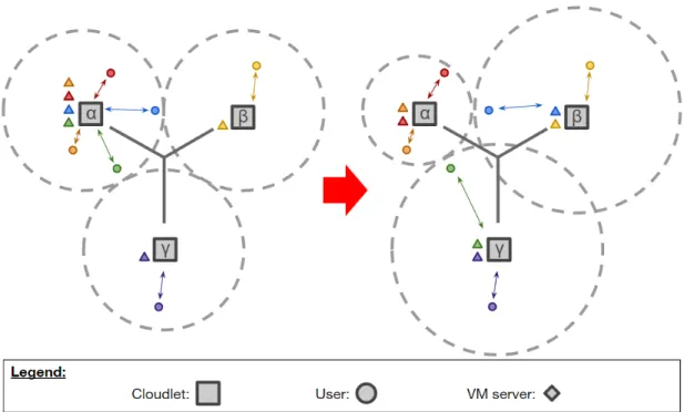
asso-ciations. c⃝ 2018 IEEE . . . 22 3.1 Illustration of Procedure 2 being executed. In the initial moment,

α is overworked while β and γ have wasted resources. After

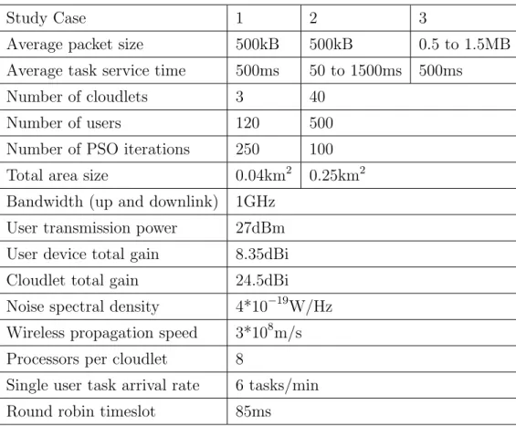
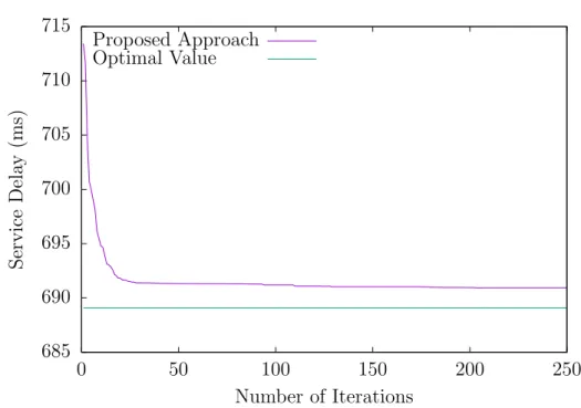
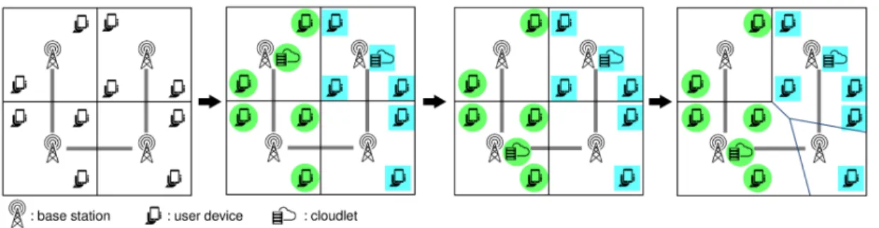
ex-ecuting the procedure, the green and blue VM servers have been migrated away from α to balance the workload, and α has lowered its transmission power level while β and γ raised theirs, to better reflect their associated users’ positions. This way, all cloudlets can efficiently reach their users, and work is equal. c⃝ 2017 IEEE . . . 45 3.2 Results for Study Case 1. c⃝ 2017 IEEE . . . 48 3.3 Results for Study Case 2. c⃝ 2017 IEEE . . . 49 3.4 Results for Study Case 3. c⃝ 2017 IEEE . . . 49 4.1 How the proposed algorithm works by assigning users to cloudlets

with kMC and then using PSO to adjust the transmission power levels. c⃝ 2019 IEEE . . . 58

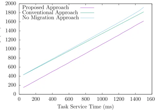
4.2 MEC service delay variation as the number of base stations is in-creased. c⃝ 2019 IEEE . . . 63 4.3 MEC service delay variation as the number of cloudlets is

in-creased. c⃝ 2019 IEEE . . . 64 4.4 MEC service delay variation as the number of users is increased.

c

⃝ 2019 IEEE . . . 65

5.1 Illustrative scenarios of how user mobility ((a) and (c)) and new users ((b) and (d)) can increase Service Delay and how cloudlet ac-tivation ((a) and (b)) and reconfiguration ((c) and (d)) can coun-teract this. c⃝ 2018 IEEE . . . 73 5.2 Maximum number of users served by our proposal with five cloudlets

under different values for PSO local inertia (ϑ). c⃝ 2018 IEEE . . 81 5.3 Maximum number of users served by our proposal with five cloudlets

under different values for PSO local acceleration (ϱh). c⃝ 2018 IEEE 82

5.4 Maximum number of users served by our proposal with five cloudlets under different values for PSO global acceleration (ϱg). ⃝ 2018c

IEEE . . . 83 5.5 Probability that latency is below the threshold based on the

num-ber of users using Application A (no relevant difference between communication or computation burdens). c⃝ 2018 IEEE . . . 85 5.6 Probability that latency is below the threshold given the number

of users using Application B (heavier burden on processing). ⃝c 2018 IEEE . . . 86 5.7 Probability that latency is below the threshold given the number

of users using Application C (heavier burden on transmission). c⃝ 2018 IEEE . . . 87 5.8 Maximum number of users for all methods under all applications.

c

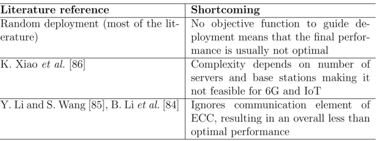
1.1 Table summarizing the main characteristics of the different cloud computing models. . . 2 3.1 Study Cases Parameters . . . 47 4.1 Existing works in ECC server deployment and what is lacking on

them. . . 54 4.2 Parameters used in the simulations. . . 62 5.1 Simulation Parameters . . . 79

Introduction

1.1

Background

Cloud Computing [1, 2] is a service model where user devices are able to connect to cloud servers. The servers have a significantly wide pool of resources (such as communication bandwidth, energy reserves/sources, processors, computing ca-pability, computer memory), a lot more than the user devices. Thus, the client devices can use those resources to execute more demanding jobs and tasks whose requirements go beyond what can be done locally by sending these tasks to the servers. The cloud denomination comes from the offloading to remote machines and the transparency of the service. Forbes [3] predicts that the cloud computing market will reach US$411 billions by 2020, and many big companies already have established cloud services, such as Google [4], Amazon [5], and Microsoft [6].

Cloud computing can work with remote servers, located far away from the user device, which could be a static desktop computer in the case of Conven-tional Cloud Computing [1, 2] or a mobile device in the case of Mobile Cloud Computing [7,8]. Mobile devices make the situation significantly different. Desk-top computers sometimes can use cabled connections to reach the cloud servers,

Category Server Location Server Capacity Number of Servers Client Profile Scenario Dynam-icity Conventional Cloud Com-puting Distant (backbone)

High Few Fixed Low

Mobile Cloud Computing

Distant (backbone)

High Few Mobile Medium

Edge Cloud Computing

Near (edge) Low Many Fixed Medium

Mobile Edge Computing

Near (edge) Low Many Mobile High

Table 1.1: Table summarizing the main characteristics of the different cloud computing models.

whereas mobile devices more often than not must depend on wireless and cellular networks in order to connect to the Internet and the cloud servers. Addition-ally, mobile devices are even more limited than desktop environments, with fewer resources and a smaller array of applications that can be executed locally [9]. This also means that they have more to benefit (i.e. the increase in the num-ber of possible applications will be bigger) from cloud computing than desktop computers. However, the need to use wireless communication and even the de-vice’s limitations complicate the deployment and the implementation of cloud computing services. To make matters more difficult, many mobile devices and mobile applications, such as Virtual / Augmented Reality programs [10], Tactile Internet applications [11], and Internet of Things (IoT) [12–14], need ultra-low latency, which cannot be possibly delivered by Mobile Cloud Computing due to the distance between the user devices and the cloud servers [15–18], which can sometimes be located in different continents [19]. To enable the execution of these applications, there have been recent efforts to create an Edge Cloud and

Mobile Edge Computing (MEC) [20, 21]1_{, where the cloud servers are, instead of}

deployed remotely, installed on the edge of the network, near the users2. In order to make this possible, there must be an edge cloud server near all users, since the main point of MEC is a close-range connection between the mobile device and the server. However, this means a huge density of cloud edge servers, which incurs an incapacitating financial cost. To counterbalance this, these edge cloud servers are designed to be less powerful than the remote cloud servers, which are more concentrated but fewer in number. Due to this smaller capacity, they have been denominated cloudlets [27, 28]. In summary, MEC offers lower latency and allows mobile devices to execute more demanding applications.

The possibility of using real-time applications and lifting device limitations has made MEC and cloudlets to be considered for future network designs along with the IoT [29–31] and 5G Networks [25]. However, there is another com-plicating issue in this caused by a key characteristic of IoT and 5G: a massive amount of devices. National Instruments estimates that 20 billions devices will be connected through 5G by 2020 [32], while Ericsson predicts 18 billion devices connected to IoT by 2022 [33]. Such scale cannot even be handled by Conven-tional Cloud Computing alone, stressing even further the need for MEC [14, 34]. But, even with low quantities of devices, many problems related to MEC are too complex to be solved [35]. With this massive amount of devices also comes a

1_{Special note here to Fog Computing [22,23], a term defined by the OpenFog Consortium [24]}

which denotes, similarly to MEC, a paradigm where cloud computation is moved closer to the origin of the data and the requests, at the edge of the network. However, Fog Computing is usually utilized specifically for deploying servers in Local Area Networks gateways.

2_{It is important to say here that MEC is also used to denote Multi-Access Edge Computing,}

a term coined by the European Telecommunications Standards Institute [25, 26] to denote the usage of edge cloud servers by mobile networks as well as Wi-Fi and other fixed access technologies. Multi-Access Edge Computing is a more broad term, encompassing Edge Cloud Computing and Mobile Edge Computing, but we opted to go with mobile over multi-access to emphasize the dynamicity of the scenarios seen in the literature. Thus, MEC in this manuscript refers to Mobile Edge Computing. Nonetheless, many of the considerations found here can be applied to Multi-Access Edge Computing as well.

great variety of services and applications. Designing a MEC environment that takes into account the various kinds of wireless characteristics, device capabilities and service requirements is yet another layer of difficulty that cannot be solved by existing solutions and heuristical algorithms [36–38].

Table 1.1 summarizes the most important points between different types of cloud computing service. Note how the location of the server and the type of device vary between them. In this research project, we will focus on MEC and how to solve its issues of problem dimensionality, number of parameters and solution executability. Nonetheless, the considerations offered here could also be applied to the other service models due to the similarities between all of them.

One alternative for dealing with these issues of parameter dimensionality and algorithm feasibility in MEC is to use Machine Learning (ML) solutions [39, 40]. The base behind ML is to allow and enable the computer program to analyze and draw conclusions on the data by itself. The program is capable of doing this by learning the intricacies of the problem it is attempting to solve and making data-driven predictions and decisions, progressively improving its performance in one pre-determined task [41, 42]. In this area, the programmer’s job is to allow the program to learn the problem (i.e. train the program), which can be done by feeding it historic input and output, or, in other words, what is the output (performance) X of solution Y given the input Z. Given a large enough amount of tuples (X, Y, Z) and a method for evaluating the value of

X, the program should be capable of drawing patterns and eventually creating

efficient solutions [43, 44]. This definition is very generic and broad and there are many variations of it, but the fundamental is the same: ML programs are capable of finding solutions that could not normally be devised (or sometimes even understood) by its programmers. These solutions, albeit not necessarily optimal, are usually efficient enough. Moreover, and more important in this

discussion, current convex optimization 3 _{techniques applied to MEC rely on}

relaxation methods in order to deal with the high dimensionality of the realistic scenarios, i.e. they cannot be applied to the original problems [35, 41], which can only be tackled by ML [45]. Besides that, ML is also a very suitable option for dynamic scenarios, since ML models can find efficient solutions even with small changes in the problem, whereas conventional approaches may need a new execution.

1.2

Research Objective

In this thesis, the main goal is to develop a framework for intelligently configuring a MEC system. Our goal will be both to increase overall quality of service as well as allow service providers to achieve a higher profit. Thus, we will minimize the service latency experienced by users, which is key for a high quality service since it makes sure that cloud computing services are transparent and the offloading to the cloud is nearly unnoticeable (i.e. it feels as if all tasks are executed locally in the user device). Besides that, a lower service delay means that users do not have to be connected to the edge cloud servers for too long, freeing up the resources so they can be assigned to new users, consequently increasing the profit of the service providers. In addition to that, we will also configure the system so that the number of users that can be serviced concurrently, while respecting a delay threshold, is maximized while utilizing as few servers as possible, thus increasing money income and decreasing costs. Moreover, as mentioned before, MEC should be utilized by a massive amount of user devices as well as many servers and access

3_{ML itself is also used for optimization. Thus, to avoid confusion, we will use ”convex}

opti-mization” when talking about the mathematical, more conventional variety of optimization and simply ”optimization” when talking about learning-based techniques for optimizing a function.

points. Thus, all these solutions will be designed with scalability in mind and should have a low execution time even with many variables. The specific MEC problems we will tackle in this thesis are listed below:

• MEC resource allocation to users • Edge server deployment policy • Server activation decision

At first, we propose a method for allocating resources from MEC to the users. This means deciding which users are assigned to which edge cloud servers in a live scenario. This should be done in a way that no server is overloaded with too many users, as that would create queues that are too long for the resources of that particular server. A similar phenomenon can be observed with base stations, as too many users connected to the same base station would create high interfer-ence and collision around that base station. Thus, our method will balance user assignment in such a way that service delay in overall is minimized.

Secondly, we present an algorithm for deciding where each edge cloud server should be deployed. The location of the servers is significant as it affects the latency needed for users to access them. We assume that servers are always deployed in base stations, since this basically eliminates the transmission between the access point and the server and base stations themselves are usually positioned in strategic places already. However, it is not economically viable nor needed to put a server in every single base station, so a policy is needed to decide which base stations receive servers. Our proposal will do that while minimizing the overall service delay.

Finally, once again in a live scenario, we propose a method for deciding which servers should be turned on and which ones can be left turned off. This allows to effectively control how many resources are present in the system. The objective

here is to utilize as few servers as possible, to lower the cost incurred on service providers. Obviously, this should be done without compromising the quality of service given to users. Thus, we establish a service delay threshold that must be respected at all times. This also allows us to guarantee to users that their service will be completed within a certain, pre-determined time window.

1.3

Summary and Organization of the Thesis

The remainder of thesis is organized as follows. Chapter 2 presents our detailed assumptions regarding the MEC system, including a mathematical model of the MEC with a formula for estimating the service delay. Chapter 3 shows our resource allocation method. Chapter 4 presents our server deployment policy method. Chapter 5 contains our server activation solution. Finally, concluding remarks are provided in Chapter 6.

Mobile Edge Computing Model

2.1

Introduction

In this section, we will present the usual MEC service model that is generally uti-lized in the literature. This service model can be configured, where configuration is the set of options and parameters that operators can decide in order to deliver the best service possible following some pre-determined evaluation. To find these optimal parameters, some challenges and problems related to MEC have to be solved; such issues are also explored in this section, but not before a presentation of existing literature works on MEC.

The contents of this chapter refer to the following papers, which were written based on our own research.

• T. K. Rodrigues, K. Suto, H. Nishiyama, J. Liu and N. Kato, ”Machine

Learning meets Computation and Communication Control in Evolving Edge and Cloud: Challenges and Future Perspective,” in IEEE Communications

Surveys & Tutorials. Available online. c⃝ 2011 IEEE

• T. G. Rodrigues, K. Suto, H. Nishiyama, N. Kato and K. Temma, ”Cloudlets

Power Control and Virtual Machine Migration,” in IEEE Transactions on

Computers, vol. 67, no. 9, pp. 1287-1300, September 2018. c⃝ 2011 IEEE

2.2

Service Model

As a prologue to the service model, it is important to explain the main enti-ties in MEC [20, 27, 28, 46]. User Device (or user) is the one who contracts the service and will create the tasks (or input, or requests) that must be executed by the MEC system; additionally, the results (or output) of the tasks must be sent back to the user device after it is done. Access Point is the device that is used by the User Device to connect to the network and reach the MEC system, such as a base station with a cellular antenna. The User Device must utilize the Access Point to communicate with the other entities and the connection be-tween Access Point and User Device is usually wireless. Cloudlet (or edge cloud server) is a physical computer that works as a server located at the edge of the network. The Cloudlet contains the resources needed for executing the requests created by the User Device. Compared to Conventional Cloud Servers, Cloudlets have lower capabilities (in computation, communication, etc.), hence their name. Virtual Machine (or virtual server) is a virtual environment located inside the Cloudlet, result of virtualization of the resources of the Cloudlet. This allows for the creation of multiple ”servers” even if there is only one single physical computer, making the separation of resources and their management easier. The Virtual Machine receives the requests by the User Device, executes the requests, and sends back the output. In order to execute these tasks, the physical server (e.g. Cloudlet) allocates some of its resources to the Virtual Machine according to the demands of the requests and a pre-determined policy. Each User Device is associated with a single Access Point, a single Cloudlet and a single Virtual Machine. Generally speaking, each Virtual Machine is only associated with one

User Device (thus, users cannot send their requests to other virtual machines, and the requests must be routed to the host of the virtual machine, regardless of where the user is and whether the user moved to somewhere since the creation of the virtual machine), while Access Points and Cloudlets can be associated with many User Devices. In physical terms, Cloudlets are usually located in the same location as Access Points, for convenience [27, 47–49]. Finally, there is also a Central Office which aggregrates important information about the system (user location, cloudlet workload, etc.) and utilizes this knowledge to make decisions and configure the system.

Also of note is that in MEC (and cloud computing as a whole), there are different products that can be offered as a service. Those are divided between Software as a Service (SaaS), Platform as a Service (PaaS), and Infrastructure as a Service (IaaS) [50]. In SaaS, the whole application is offered by the cloud service provider, and the users just supply the data that serves as input and in return receive the corresponding output [51]. In PaaS, the service provider offers everything up to the operating system and the client provides the application that will be executed [52]. Thus, in PaaS, the user will send both its application and the input for it, the application will utilize the cloud resources, and then the user will collect the output. Finally, in IaaS the service provider makes available to the user its computers, storage, networking equipment through virtualized resources that the client can acquire as needed, while the user is responsible for deploying everything from the operating system onward [53]. In other words, the user provides and manages the platform, which will be run on top of the service provider’s resources. Note, however, that all these models operate with virtual servers on top of the physical resources from the provider, as shown in Figure 2.1. Thus, the structure based around the virtual server described previously can still be applied to MEC regardless of the product being offered.

Processors

Storage

Network

Virtual Server

Operating

System

Application

Input (tasks)

Processors

Storage

Network

Virtual Server

Operating

System

Application

Input (tasks)

Processors

Storage

Network

Operating

System

Application

Input (tasks)

SaaS

PaaS

IaaS

Serv

ice

Pr

ovid

er

Use

r

Virtual Server

Figure 2.1: Comparison between SaaS, PaaS, and IaaS, specially in what is offered by the users and what is offered by the Service Providers in each service model. c⃝ 2019 IEEE

The MEC service model is usually assumed to be as follows [21, 27, 54–58]. When first entering the system, the user device makes an initial request that is received by the closest cloudlet. This request may be forwarded to a remote centralized entity (a central device with full information and control of the MEC system) or resolved in that edge cloud server. The result of this request is the creation of a Virtual Machine which will serve that user1 _{(realistically speaking,}

1_{The Virtual Machine is intrinsically connected to the service provided. Thus, if MEC is}

offering a specific application as a service, the Virtual Machine is capable of performing any routines related to that application. Conversely, if the platform or infrastructure is offered as

Figure 2.2: Diagram illustrating a generic view of the service model in MEC (although Access Point and Cloudlet are virtually different entities, they are usually physically together and always at the edge). c⃝ 2019 IEEE

there is an overhead related to virtualizing the resources of the host server when creating the virtual machine, which delays the beginning of the service by an

amount that varies depending on what exact service is offered [59]). As for what this service entails, it depends on the application, but it could go from task offloading and extending the environment of the user to even content delivery and caching, as mere examples. This virtual server will be hosted by one of the cloudlets of the system, with the choice of which one being made following a pre-determined policy. After this initial setup, the user will proceed to send tasks to its corresponding virtual server, who will receive this input and process them utilizing the local resources of the edge server. After finishing execution, the virtual server sends the output of the task back to the device, which displays it to the user as if it was a terminal. This communication between user device and edge cloud / virtual server happens wirelessly between the device and the access point and through a cable between the access point and the edge server. Figure 2.2 shows a diagram illustrating a typical MEC service model and all of its entities (note how the virtual server is inside the cloudlet). There are some relevant variations to this model, with the most prevalent being: multiple virtual servers [60,61], task fragmentation [62,63], virtual server migration [54,64], cooperation with remote servers [65, 66], and virtual containers [67, 68].

As a minor sidenote, one service model variation that deserves more attention is user mobility. The decision to consider user movement in the assumed scenario can indeed increase significantly the difficulty to solve a problem [69]. The issue comes from the uncertainty and dynamicity created by user mobility since the channel proprieties are always at risk of changing due to the user moving [49, 61, 70]. This movement could simply put more distance between the user and the access point, decreasing signal quality due to path loss, or even put the user in an area with more interference and obstacles. Consequently, it is very much a possibility that the user will transition to a state where a new access point is more favorable, which further complicates things with handover between the base

stations. Moreover, it may also mean that the user suddenly benefits more from connecting to a new edge server. Finally, all these changes are very difficult to predict, even if the users are assumed to follow some mobility models. Thus, a lot of MEC research prefers to ignore user mobility altogether [62, 65, 71], which is an option albeit not the best one in terms of choosing a realistic scenario.

As it is evident from the model and regardless of variations, service in MEC can be divided into two main segments: the transmission element (the communi-cation between the user and the cloudlet) and processing element (the execution of the request sent by the user to the cloudlet) [21, 54, 55]. In the communica-tion side, performance is mainly affected by interference between devices, band-width available, physical propagation, noise, transmission power and payload size [13, 62, 70, 72]. Meanwhile, in the computation side, performance mainly de-pends on server processing speed, size of the task (number of instructions, cycles required, etc.) and the competition for server resources [66, 73–75]. Some MEC applications will generate heavier communication payload (e.g. content delivery, where users may download videos and pictures that will put a lot of stress in the network), some MEC applications need to execute many instructions for their requests and will demand a lot of time from the processors at the cloud servers (e.g. image processing, where the images sent by the user devices must be fully analyzed while looking for points of interest), while some other MEC applica-tions are a mix of both (e.g. big data analytics, where big databases must be transmitted and then analyzed at the processors). These show examples of high communication burden and high computation burden among MEC applications. These different profiles and requirements further complicate MEC operation, as the applications will need different resources and systems if an efficient service is desired (e.g. for content delivery, investment in bandwidth is desired, while for image processing, investment in more capable servers is desired; for servicing

both simultaneously, either the network is heavily and expensively equipped or the algorithm must be very efficient in resource allocation, which is obviously preferred) [76].

Additionally, it is worth noting that the service model in MEC is virtually identical to the one in Mobile Cloud Computing and Conventional Cloud Com-puting, involving Virtual Machines and job offloading. Consequently, many of the design and implementation problems in Mobile Cloud Computing and Conven-tional Cloud Computing are similar to what we find in MEC. However, there are some key differences. Firstly, due to lower latencies, MEC can service real-time applications and devices that demand quick response times on top of all applica-tions and devices that conventional cloud computing handles, meaning that MEC has to work with a higher variety and bigger amounts of clients. Secondly, not only there are more clients, mobile devices themselves have features that cannot be ignored which may make local processing impossible or at least undesirable, such as their battery level, memory, and transmission data rate [31]. Those resources are particularly limited in mobile devices and their availability may change over time, which makes decisions on offloading, for example, even more complicated. Also, MEC also has to work with many more servers (actually, the concentrated servers in Mobile Cloud Computing can even be considered as one single giant server [77]). Finally, the networks in the edge are much more dynamic. These characteristics mean that problems in MEC have more parameters, higher dimen-sionality and incur higher volumes of data. For these reasons, solutions used in Mobile Cloud Computing / Conventional Cloud Computing often do not apply to MEC.

2.3

Challenges

With an objective function (or a combination of more than one [62, 78]) chosen, the cloudlet or the central office of the MEC service must then decide which configuration to utilize in order to optimize this objective. This configuration must answer possible questions regarding the service model of the system (e.g. which cloudlet will host the virtual server, which jobs will be offloaded). In the literature, this translates to a set of problems that are solved in order to raise the efficiency of the MEC system. These problems are usually independent of service variation or objective function. In the following sub-sections, we present categories of notable MEC problems.

2.3.1

Offloading Decision

Given one of the objectives previously mentioned, the class of problems related to offloading decision decides where the user-generated tasks should be executed. The choices can be local, inside the user device itself; the edge cloud servers, located near the user, following MEC; and the remote conventional cloud servers (as in Mobile Cloud Computing). In case of choosing the edge cloud servers or the remote cloud servers, a second possible choice is which server will execute the task, although this can be omitted in both cases (e.g. no virtual server migration so the host server is already decided; the remote cloud servers operate jointly as a massive super server [73, 77]). Moreover, the whole definition of the user task can vary between works, whereas some consider solid, indivisible tasks [73,79] while others fragment them into subtasks (that can be dependent or independent between themselves) [62] and some others even duplicate tasks for redundancy [80]. Despite all these possible variations, the pattern is the same: decide where the user-generated task will be executed such that the objective function is optimized. Research work in this area usually concludes that offloading

decision (even in simplified scenarios with a single user or a single server) is either NP-hard [62] or NP-complete [73], such that relaxation or heuristic algorithms are usually the proposed solutions. However, such algorithms have their complexity order proportional to both the number of devices and servers, which renders them unfeasible in the future networks with massive amounts of agents.

2.3.2

Resource Allocation

Even if the offloading target is decided, service may be affected and changed by allocating more or fewer resources to the user. Because in real-life situations, both the user and the cloud server, either at the edge or at a remote location, have a limited amount of resources, the decision of how many to allocate to the MEC service is an important one in order to operate the network efficiently and to unleash the full potential of the system [65]. This resource allocation can be done either in the fronthaul, i.e. directly involving the user and its relation with the rest of the system, or in the backhaul, i.e. without direct relation to the user. The resource allocation decision can be made by a centralized office, with full [65,74] or partial knowledge [81] of the system, or individually by each server / user device [13,82]. These resources are mostly related to the communication side (sending input and output between the user device and the server), although there are some mentions to the applicability in the computation side (the execution of the task). For communication, examples are channel bandwidth [65, 74] and transmission power [54, 55], among others. All these affect the communication latency between the user and the server, so they consequently have effects on the service latency. Transmission power has a direct effect on the energy consumption of the nodes, while the communication delay itself has an indirect consequence in that the nodes may have to spend more time transmitting. The same can be said about profit, relating the money spent on energy and the monetary gain by

finishing more tasks in less time. Regarding resources in the computation side, notable examples are number of processors in a single server [65, 74] and even the speed of these processors [62], although research involving such parameters is rather scarce. Specifically related to backhaul resource allocation, notable mentions are servers sharing workload [72], servers sharing resources [83], virtual servers being migrated [61, 70], among others. The problem of deciding how many resources to allocate in order to optimize a system-wide metric is also usually solved by heuristic algorithms that are usually more complex if the model of the scenario is more realistic. Furthermore, since this allocation is taken with a system view, it is also affected by the number of devices and servers, which renders them unfeasible in the future networks with massive amounts of agents.

2.3.3

Server Deployment

A problem that is very characteristic of MEC is the choice of where the servers will be deployed. Being edge servers, there are usually multiple choices of where they could be installed. As mentioned before, they are typically located near network access points, but since it is not viable or necessary to have one server in each access point, there is still a choice to be made [47,48]. The conclusion is that there must be a choice of where to deploy the servers, which naturally should be guided by an objective function, trying to optimize a pre-determined goal, such as the ones listed in our previous sub-section. This usually means deploying servers near places where users conglomerate, so more clients can be served (raising profit) with shorter connection distance [48, 84]. However, in MEC particularly, users can move, which may turn a deployment location from a desirable one into a bad position [49]. Moreover, differently from virtual machines, server deployments are usually permanent, or at the very least expensive to change, demanding extra care when choosing. Furthermore, the deployment choice also comes with important

financial consideration, as the number of servers and their locations all come with associated costs [85, 86]. The deployment places may have to be rented or equipment has to be acquired, making this an essential consideration even if the objective function is not based on the service provider’s profit. From this discussion, it is clear that solutions to the deployment challenge depend heavily on how many servers will be deployed and how many choices are there, which in itself already means a complex scenario. Furthermore, the dynamicity of MEC means that the scenarios keep changing, which comes in contrast to the permanency of the deployment decision, making the choice of a good location even more difficult, especially in a future with the massive amount of servers and devices to be served.

2.3.4

Overhead Management

Finally, another point of note is how all these configurations and actions incur significant overhead. The choices of where to offload and how many resources to allocate are all performed online, meaning that until such decisions are made, the received requests will not be processed nor answered, increasing the latency and decreasing service quality [87,88]. Moreover, there are other actions in the service model of MEC that result in overhead as well, particularly the ones related to the virtual server. Not only a choice has to be made of which physical server will host the virtual server for each client, the virtualization process itself and the initial setup of the virtual server takes time [59]. Additionally, in scenarios with virtual server migration, this transfer of the virtual machine between servers also takes time, during which the service is potentially paused [60]. Other possible causes for overhead cost include handover between networks when the user moves [89,90], orchestrating the cooperation between different domains [19,72], deciding the routing between the user device and the associated servers [91, 92], among others. Most works tend to ignore some if not all of these overhead sources,

but for a more realistic modeling of the scenario, they should be considered. However, not only the calculation of overhead itself is quite difficult, overhead costs themselves will probably ramp up as more devices and more servers are considered since these extra agents mean more complications for the algorithms responsible for calculating the configurations, which means they will take longer to execute [36, 38].

2.4

Mathematical Model

In this section, we will present a mathematical model for calculating the estimated average Service Delay in MEC as a function of time and the scenario scale (i.e., the number of users). We will begin by presenting our assumed scenarios. Then, we will model user mobility and how to calculate the number of users associated with each cloudlet. Finally, we will present equations for calculating Transmission Delay, Processing Delay, and Backhaul Delay before joining the entire model into a calculation of the average Service Delay.

2.4.1

Assumed Scenario

For starters, we will discuss several assumptions about our scenario. We have a bounded area A (where A denotes the area and its size in square meters). Inside this area, we have the cloudlets and the clients that will be associated with them.

λ(X, tk) denotes how many users are in point X at timeslot tk. Therefore, users

are initially disposed in A following a density function λ(X, 0). However, users are mobile and can roam from this positions to any point inside of A. Furthermore, to symbolize a growing demand, we have that at timeslot tk, α(X, tk) new users

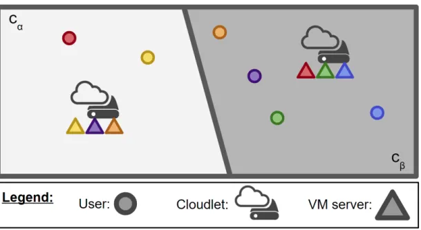
appear in point X, where α(X, tk) is our spawning function. We assume this

Figure 2.3: Illustrative example of six users and two cloudlets and their associa-tions. c⃝ 2018 IEEE

under extreme stress conditions; if they behave well in this scenario, they are able to handle simpler cases as well [139]. There are|C| cloudlets in the scenario, which all belong to set C; we denote them by ci, with 0≤ i < |C|.

For now, we will assume that all base stations have a co-located cloudlet. This allows us to treat cloudlets both as servers and as base stations. Users have a physical and a virtual association [93]. The physical association determines with which cloudlet they communicate through a direct wireless connection. The user will send their tasks and receive output from this cloudlet. The virtual association determines which cloudlet will host the VM server associated with the user that will actually execute the tasks created and produce the output. If a user is physically associated to cloudlet ci and virtually associated to cloudlet

cj, then ci and cj will communicate through a backhaul link to exchange the task

the user by ci). We assume there is a switch in the backhaul that connects all

cloudlets, and each cloudlet has a physical link connected to this switch [94]. Physical association is decided by RSS, where clients will always associate with the cloudlet that currently offers them the highest RSS value. This means that area A will be divided following a Voronoi diagram between the cloudlets. However, unlike conventional Voronoi diagrams, the subareas are decided based on RSS instead of only Euclidean distance. Therefore, area A is divided into|C| subareas Aci, where all users inside Aci are associated with and will send tasks to

cloudlet ci. If a user leaves Aci and goes into Acj, then its physical association is

changed from ci to cj. The virtual association is determined by the initial position

of the user only, i.e. the user will virtually associate with the cloudlet that offers the highest RSS at the timeslot the user shows up in the system. Even if the user moves, its virtual association (the host of its VM server) will not change.

As mentioned, λ(X, tk) defines how many total users are in X in timeslot tk.

All these users are physically associated to ci if X ∈ Aci, but λ(X, tk) tells us

nothing about their virtual association. Therefore, let us define a new density function λci(X, tk) that represents the total number of users virtually associated

to cloudlet ci that are located in X at timeslot tk. Note how λci(X, tk)≤ λ(X, tk).

Figure 2.3 illustrates the difference between those two values. Here, Acα is light

gray and Acβ is dark gray. In the light gray area,

∫∫

λ(X, tk)dX is two because

there are two users in that region, the red user and the yellow user, who are represented by circles. Also in the light gray area,∫∫ λcα(X, tk)dX is one instead

of two because, of the two users in that area, only one user (the yellow one) has its VM server (represented by the triangle) hosted by cα. Analogously, in the

dark gray area,∫∫ λcα(X, tk)dX is two because two users in that area (the purple

and orange ones) have their VM servers hosted by cα; these users are not in the

link and cβ as a relay to reach their VM servers.

If Service Delay increases too much (for example, because of an overload on the backhaul caused by mobility) and goes beyond the acceptable limit, the system enters a Configuration Phase. For example, transmission power levels can be changed to create a more efficient cloudlet configuration. Physical and virtual associations are then reset to the new resulting RSS Voronoi Diagram, which may lead to VMs being migrated.

For this mathematical model, we will denote initial moment as t0, which

rep-resents the initial moment of any cloudlet configuration. This can mean either the beginning of the service, or after Virtual Machines are migrated, or after a new cloudlet is activated. Basically, t0 means the timeslot after a new

config-uration of transmission power levels is set (with the possibility of VMs having been migrated) and the virtual association of the users follows the RSS Voronoi Diagram. As a final note, it is important to say that some variables here are calculated at each timeslot while others are calculated only once considering the initial user distribution. This was chosen for simplicity, because calculating every single variable for all timeslots would be too complex. The selection of which variables would be considered was based on how susceptible they are to changes in the number of users. For example, variables related to queues vary exponen-tially with number of users and arrival rate. This variation is also relevant to the migration of users.

2.4.2

User Mobility

We assume users move thusly [95]: the time dimension is divided into timeslots with equal length T; at each timeslot tk, each user chooses a random direction

and moves towards it with speed dictated by a probability density function ζ() (maximum speed is v). Each direction has an equal chance of being selected, so

the probability that a particular direction is picked is _2π1 .

Therefore, the expected value of λ(X, tk) (and λci(X, tk)) is determined by

how many users ended in point X at the end of timeslot tk. To calculate such

number, we utilize a double integral using the number of users at the previous timeslot, the odds of those users picking the direction of X, and the odds of the users picking the speed that will land exactly into X at the end of the timeslot, over the area dictated by Ω(X), which is a circle with a radius of Tv and centered in X. Additionally, we must also consider the users that spawned in the point in this timeslot (α(X, tk)). Here, rYX is the Euclidean distance between X and Y ,

and αci(X, tk) is analogous to α(X, tk), but considers the spawning of users that

are virtually associated to cloudlet ci only (αci(X, tk) is equal to α(X, tk) if X

is inside the association area of ci; i.e. the area where ci offers the highest RSS

among all cloudlets, denoted by Aci; and it is zero otherwise).

E[λ(X, tk)] = α(X, tk) + ∫∫ Ω(X) ( 1 2πζ ( rY X T ) λ(Y, tk−1) ) dY (2.1) E[λci(X, tk)] = αci(X, tk) + ∫∫ Ω(X) ( 1 2πζ ( rY X T ) λci(Y, tk−1) ) dY (2.2)

2.4.3

Number of Users

As previously mentioned, the number of users in an area Aci at timeslot tk is

determined by the expected value of λ(X, tk). Therefore, if UA_ci(tk) is the number

associated to cloudlet ci at tk), then we can find this value by calculating the

double integral of λ(X, tk) over the desired area.

UA_ci(tk) =

∫∫

A_ci

E[λ(X, tk)]dX (2.3)

The number of virtually associated users, i.e. the number of Virtual Machines receiving new tasks inside of cloudlet ci, in instant tk is determined by Vci(tk) in

an analogous way but using λci(X, tk) instead.

Vci(tk) =

∫∫

A_ci

E[λci(X, tk)]dX (2.4)

2.4.4

Transmission Delay

We assume that the channel capacity for transmission follows the Shannon Hart-ley theorem [96], shown below. Here, C is the channel capacity (bits per second), B is the channel bandwidth (Hertz), S is the RSS (Watts), N is the Additive White Gaussian Noise [97] spectral density (Watts per Hertz) and I is the sensed interference (Watts). C = Blog₂ ( 1 + S BN + I ) (2.5) Additionally, we have the formula for RSS below, for a transmitter aT X and a

receiver aRX. The formula calculates the signal power in decibels through the

transmission power (ωaT X), the antenna gains at both nodes (GaT X and GaRX),

the Rayleigh power fading constant (H, which is the value corresponding to 0.5 in the cumulative distribution function for average [98]) and the path loss between

both nodes (LaTX

aRX), all given in decibels. It then converts this value to Watts.

SaTX

aRX = 10(

ω_aTX+G_aTX+G_aRX+H−LaTX_aRX)10

/1000 (2.6) Path loss is given by the Dual Path Empirical Path Loss model, shown below for a transmitter aT X and a receiver aRX. Here, raaRXTX is the distance between the

transmitter and the receiver, n1 and n2 are the path loss constants for short and

long distance, respectively, and rb is the breakpoint between both classifications.

LaTX aRX = L1+ 10n1log10r aTX aRX + 10(n2− n1) ( 1 + r aTX aRX rb ) (2.7) The Transmission Delay for each task is given by the average time needed to traverse the distance between user and cloudlet twice (once for downlink and once for uplink), where the average distance for clients of cloudlet ci is gci and the

propagation speed is γ; the average time needed to send a packet in the uplink at instant tk (Dcupi(tk)); and the average time needed to send a packet in the

downlink (Ddown

ci ). Thus, the average Transmission Delay for clients of cloudlet

ci in timeslot tk is given by ˙ Tci(tk) = 2 gci γ + D up ci (tk) + D down ci (2.8)

In order to find gci, we utilize another double integral with the density function,

but this time utilizing the distance between the point and cloudlet ci. Again,

because this is an average, we must divide by the total amount of users.

gci = ∫∫ A_ci ( λ(X, 0)rX ci ) dX ∫∫ A_ci λ(X, 0)dX (2.9)

In the uplink, we can calculate the average time needed to send a packet through (2.5) by using the average size of an uplink packet, denoted by pup _as

shown below. Here, Bup _{is the uplink bandwidth (in Hertz) and I}

ci is the

inter-ference suffered by cloudlet ci, which is the receiver used here. Once again, we

utilize a double integral to obtain the value for all users in the area and divide the value by the total number of users to find the average.

Qup_c i = ∫∫ A_ci  λ(X, 0) pup Bup_log 2 ( 1+ SXci BupN +Ici )   dX ∫∫ A_ci λ(X, 0)dX (2.10)

For the uplink, we assume users of the same cloudlet follow round-robin scheduling [99] to send their packets. This eliminates collision between users of the same cloudlet, but still leaves the possibility of interference from users of other cloudlets who may be transmitting at the same time. However, because they also follow round-robin scheduling, only one user from each other cloudlet could cause this interference. To calculate the average interference sensed by ci, we must calculate

the average signal power received from users of each of the other cloudlets and sum these values. This value is found by taking a double integral of the total signal power generated by all users, and dividing by the number of users for average, as shown below.

Ici = c∑j̸=ci cj∈C     ∫∫ A_cj ( λ(X, 0)S_cX_i)dX ∫∫ A_cj λ(X, 0)dX     (2.11)

If the users follow a round-robin scheduling, then they follow an M/D/1 queue model [99, 100], where 1 represents the single channel for transmission, D means that the timeslot size is a constant value (τ ), and M represents the Poisson process that users follow when generating new packets (tasks) and putting them in the queue while waiting for the channel to be available. The average rate of this process is determined by the average task generation rate for a single user

(denoted by Λ1) multiplied by the number of physical users currently associated

to ci in instant tk, with the addition of users that did not finish sending their

packets at the current timeslot. This last value can be calculated as follows. We first calculate the chance that the user will finish in the current timeslot by dividing the length of the timeslot (τ ) by the total time needed (Qup

ci). Because we

want the opposite of that (the chance that the user does not finish), we subtract such value from 1; this gives us the rate of users that do not finish per timeslot, so we divide that by the length of the timeslot to obtain the value at users per second. It is noteworthy how this value is only applicable if a single timeslot is not sufficient to send a packet; otherwise, it is ignored. Finally, the formula for the arrival rate of packets at this queue for sending to cloudlet ci at instant tk is

given by ϕci(tk) =      Λ1Uci(tk) + 1− τ Qup_ci τ , if Q up ci > τ Λ1Uci(tk) , otherwise. (2.12)

From this value, the average wait time in the uplink queue for clients of cloudlet

ci at instant tk follows immediately from queuing theory and is given by

ϖci(tk) =

ϕci(tk)τ

2

2(1− ϕci(tk)τ )

(2.13) Finally, to calculate the total time spent to send a packet in the uplink, we must first determine how many timeslots are necessary by using Qup

ci and τ . Because

all timeslots involve a waiting time prior to obtaining the channel for the length of the timeslot, we multiply that latter number by the sum of the wait time and

τ , which leads us to the formula below. Dup_ci (tk) = ⌈ Qup_ci τ ⌉ (ϖci(tk) + τ ) (2.14)

For the downlink, we assume that each user is allocated a fraction of the total bandwidth through OFDM [101]. This allows us to concurrently transmit to all users of a single cloudlet without worrying about collision (because the frequency bands are different). We can also utilize this to implement fairness into the model by allocating wider bandwidths to users in less favorable locations (i.e., ones that receive a weaker RSS). To do so, we allocate bandwidth to each user that is proportional to the ratio of the inverse of the logarithm base 2 of the RSS it receives from its cloudlet when compared to the sum of the same value for all users of that cloudlet (this value is obtained through a double integral that involves the density function and the corresponding area). Because we use the inverse, users with higher RSS will get less bandwidth, and vice versa. Thus, assuming that X0 ∈ Aci and B

down _{is the total downlink bandwidth (Hertz), the}

bandwidth allocated to a user in X0 is

bdown_X 0 = B down ( Sci X0 )−1 ( ∫∫ A_cj (λ(X, 0)Sci X) dX )₋₁ (2.15)

Here, although transmissions to clients of the same cloudlet do not interfere with each other, there is still interference coming from the other cloudlets. This occurs because there is no coordination between cloudlets, so they do not allocate the same wavelengths to their users. Therefore, we calculate the interference at that previous user in X0 associated to ci by summing the RSS received by the other

cloudlets. IX0 = c∑j̸=ci cj∈C Scj X0 (2.16)

Finally, the average total time for transmission in the downlink is calculated in the same way as performed in (2.10), but using the average packet size for

downlink (pdown_{), and the new values for bandwidth ((2.15)) and interference} ((2.16)) instead. Ddown_c i = ∫∫ A_ci  λ(X, 0) pdown bdown_X log2 ( 1+ S ci X bdown X N +IX )   dX ∫∫ A_ci λ(X, 0)dX (2.17)

These formulas allow us to calculate the average Transmission Delay at times-lot tk for all users in the system. This is accomplished by utilizing the average for

the users physically associated to each cloudlet, multipliying by the number of users physically associated to that cloudlet, and then dividing the sum of those numbers by the total amount of users for averaging.

Tdelay(tk) = ∑ ci∈C ( UA_ci(tk) ˙Tci(tk) ) ∑ ci∈C UA_ci(tk) (2.18)

2.4.5

Processing Delay

We assume that the access to the processors at each cloudlet follows an M/M/k queue [100], where k is the number of processors for each physical cloudlet, the individual processing time for the tasks comes from a Poisson process with average

µ, and tasks arrive following yet another Poisson process. The rate for this former process comes from the average task generation time of a single user (Λ1)

multiplied by the total amount of VM servers hosted by cloudlet ciat that timeslot

(Vci(tk)). The total arrival rate at timeslot tk for cloudlet ci is given by

Λci(tk) = Vci(tk)Λ1 (2.19)

tk can then be derived by

ρci(tk) =

Λci(tk)

kµ (2.20)

From this, the chance of waiting in the processors’ queue at cloudlet ci at instant

tk also comes instantly from queuing theory.

Ψci(tk) = (kρci(tk)) k k! ( (1− ρci(tk)) k−1 ∑ n=0 (kρci(tk)) n n! + (kρci(tk)) k k! )−1 (2.21)

Because queuing theory also gives us the average waiting time for these users of cloudlet ci at instant tk based on the previous variables (the first factor of the

right-hand side in the formula below), we can calculate the average Processing Delay for the clients of cloudlet ci at timeslot tk by adding this value to the

average time needed to process each task.

˙ Pci(tk) = Ψci(tk) 1 1− ρci(tk) 1 kµ + 1 µ (2.22)

Finally, the average Processing Delay for all users in the system can be obtained in the same way that (2.18) was calculated.

Pdelay(tk) = ∑ ci∈C ( Vci(tk) ˙Pci(tk) ) ∑ ci∈C Vci(tk) (2.23)

2.4.6

Backhaul Delay

As mentioned before, all cloudlets are connected to a backhaul switch [94]. This connection is comprised of|C| fiber optic links (one for each cloudlet, connecting them to the switch), and it is used when a user is physically and virtually asso-ciated to two different cloudlets. Let us consider cloudlets ci and cj. Through

Wavelength-Division Multiplexing (WDM) [102], a dedicated wavelength is re-served in the links connecting ci and cj to the switch; this band will be used

exclusively for backhaul communications between these two cloudlets, i.e., by users who are physically associated to ci and virtually associated to cj or

vice-versa. Let us assume this band has a length of Rci,cj (the order between ci and

cj is irrelevant here), where, for all pairs of cloudlets in C, Rci,cj Hz are reserved

exclusively for that pair. These Rci,cj Hz are equally divided between all users

(and their VMs) of that pair of cloudlets who need it (users virtually associated to

ci located in Acj and vice-versa). Thus, we have that, for the pair ci and cj, users

will have the following bandwidth available to them for backhaul communications during timeslot tk. rci,cj(tk) = Rci,cj ∫∫ A_ci E[λcj(X, tk)]dX + ∫∫ A_cj E[λci(X, tk)]dX (2.24)

Such bandwidth is utilized both for sending the input packet (from the user to its VM) and the output packet (from the VM to the corresponding user) between both cloudlets. Sending such packets through this dedicated wavelength band is what creates the backhaul delay. Below is a calculation of the average backhaul delay across all users during timeslot tk. Note how even though the delay is only

average considers the total amount of users. Bdelay(tk) = ci∑̸=cj (ci,cj)∈C2 ( ∫∫ A_ci E[λcj(X, tk)]dX pup_+pdown r_ci,cj(tk) ) ∑ ci∈C Vci(tk) (2.25)

2.4.7

Service Delay

Finally, Service Delay can be calculated at each timeslot by adding the delays related to transmission, processing, and the backhaul.

Sdelay(tk) = Tdelay(tk) + Pdelay(tk) + Bdelay(tk) (2.26)

2.5

Summary

This chapter offers important considerations for modeling problems in MEC. This includes a basic service model, with its entities and variations. More importantly, this chapter presents broad categories of MEC challenges, which are a useful start-ing point for research. In this sense, it is important to also discuss what are the current directions and trends in each challenge. For example, in the Offload-ing Decision category, the final goal is obviously to utilize multiple and various servers, in the edge or not, as possible destinations [9, 27]. This means a lot of variables to consider, as discussed previously. Compounded by a high quantity of users, the resulting problem ends up being very difficult to solve. Thus, more and more literatures pieces published recently are using a user-centric approach, where they focus on solving the problem for a single user [82,103,104]. This means a simpler (and thus feasible) solution that could be applied in a user-by-user case. This idea is also applicable to and can be seen in resource allocation, both in the fronthaul and the backhaul [105, 106]. However, for resource allocation, it is also

notable how more and more research is being made combining both the Com-munication and Computation planes of the service model [81, 107]. Previously, a lot of MEC work would focus on a single aspect, e.g. how to minimize the transmission delay, how to maximize processor utilization [13]. However, both transmission and processing are important for the quality of service and they are also dependent on each other, so much so that modifying communication parameters will affect the computation part of MEC. Thus, it is necessary when building a realistic solution to consider the whole service model of MEC, despite how complex this is [76]. In the case of Server Deployment, it is interesting to investigate other deployment locations besides next to base stations. Obviously, this comes with the drawback of the connection between the edge server and the base station, to integrate it with the network, which must be considered in the final model and objective function. Nonetheless, there are some benefits to this, as there may be locations with lower monetary costs (e.g. cheaper rent) or better energy infrastructure to set up the edge servers, bringing benefits to the service provider [108]. Moreover, there can be already existing servers that perform dif-ferent, local functions in the edge (e.g. servers in a company or university) that could secondarily be utilized as MEC servers [27]. These possibilities are not very touched in the literature. Finally, Overhead Management as a whole is not studied enough, so there is plenty of work that could be performed in this field yet [87, 88]. The estimation and calculation of the overhead cost associated with each action and the integration of this with the other decision (e.g. the offload-ing destination or resource allocation ones), includoffload-ing its impact in the objective function, are useful future perspectives. This goes especially in contrast with the many research works that mainly assume that their proposed solutions will either be performed offline always or will have negligible cost, which is not realistic in most scenarios [87, 88, 90]. Finally, the chapter concludes with a mathematical

respresentation of the assumed MEC model. This includes a method for estimat-ing the service delay of the system, includestimat-ing the latency needed for processestimat-ing the user-generate tasks and transmitting them from the users to the access points and from the access points to the cloudlets.

Machine Learning-based

Resource Allocation

3.1

Introduction

In this chapter, we propose a method for lowering both Processing Delay and Transmission Delay in a scenario with an undetermined amount of cloudlets. The proposal utilizes Virtual Machine Migration to move Virtual Machines related to users from one cloudlet to another, and Transmission Power Control at the base stations to determine the signal strength received at the users and thus the communication quality. Those main technologies are used for achieving the following goals: effectively lower Service Delay as much as possible, provide a high Quality of Service for various application profiles, and stay computationally feasible. We utilize a mathematical model with a Particle Swarm Optimization (PSO) model [109], a Machine Learning technique, to achieve a low execution time and high efficiency.

The contents of this chapter refer to the following papers, which were written based on our own research.

• T. G. Rodrigues, K. Suto, H. Nishiyama and N. Kato, ”Hybrid Method for

Minimizing Service Delay in Edge Cloud Computing Through VM Migra-tion and Transmission Power Control,” IEEE TransacMigra-tions on Computers, vol. 66, no. 5, pp. 810-819, May 2017. c⃝ 2011 IEEE

• T. G. Rodrigues, K. Suto, H. Nishiyama and N. Kato, ”A PSO Model with

VM migration and Transmission Power Control for Low Service Delay in the Multiple Cloudlets ECC Scenario,” in Proceedings of the 2017 IEEE

International Conference on Communications (ICC), Paris, pp. 1-6, May

2017. c⃝ 2011 IEEE

3.2

MEC Resource Allocation in the Literature

As mentioned before, the main requirement in MEC, to lower the Service Delay, can be translated to lowering the Transmission Delay and the Processing Delay. We define Transmission Delay as the time required for the user to send its task to the cloudlet plus the time it takes for the cloudlet to send this task’s output back to the user. Since these actions are performed in the wireless medium, it is straightforward that parameters related to the wireless environment are the ones who affect this delay. Meanwhile, we define Processing Delay as the time required, inside the cloudlet, for the task to be executed and its output to be produced. This involves the time the task spends in the processor queue, waiting for access to the processor, as well as the time the processor takes to actually execute the task. Therefore, this type of delay is intrinsically connected to the efficient utilization of the processors of the cloudlets. Finally, we define Service Delay as the simple sum of the Transmission Delay and the Processing Delay. Through this division, we can separate existing approaches to handle the Service Delay requirement in the literature into two classifications: those related to Processing Delay, and those

related to Transmission Delay.

In the computation side, existing methods for lowering Processing Delay are mainly based on balancing the workload between the physical cloudlet servers, attempting to avoid overwork and/or wasted resources in any of the cloudlets. Since such goal leads to efficient use of the processor resources, it is an effective way of controlling Processing Delay. This can be achieved by always associat-ing new users with cloudlets that currently have the least amount of work, in a technique called Work Scheduling [110, 111]; this would balance the workload and guarantee that the difference in amount of hosted Virtual Machine servers between cloudlets is minimal. Another existing approach, called Virtual Machine Migration [112, 113], deals with fixing situations where the workload is already unbalanced; it is based on migrating Virtual Machine servers from busy cloudlets to underworked ones, avoiding the wasting of resources on the latter group and keeping the workload more balanced. Finally, one other possibility is to divide the task into mutually independent components that can be executed in parallel; some of these components are executed locally, in the mobile device, while others are offloaded to one or more cloudlets. This technique, called Application Par-titioning [114–117], is based on deciding which components to offload and which cloudlets should be their destination, with the choice being based on minimizing Processing Delay by avoiding sending requests to servers that are already over-worked and would take longer to execute the task than the mobile device, and also spreading your components so that no single server is overwhelmed.

As it was mentioned before, Transmission Delay is closely connected to the wireless medium where the transmission is performed. For this reason, approaches focused on communication elements mainly concentrate on metrics such as Signal to Interference plus Noise Ratio (SINR), latency, and throughput. One existing technique is called Access Point Scheduling [118, 119], where users are associated