東北大学機関リポジトリTOUR

(1)

Poverty Dynamics and Poverty Reduction in

Ethnic-minority Areas of Northwest China

著者

Wang Longkui

学位授与機関

Tohoku University

学位授与番号

11301甲第18937号

(2)

POVERTY DYNAMICS AND POVERTY REDUCTION

IN ETHNIC-MINORITY AREAS OF NORTHWEST CHINA

（中国西北少数民族地域における貧困動態と貧困削減について）

A DISSERTATION SUBMITTED TO THE GRADUATE SCHOOL OF

AGRICULTURAL SCIENCE, TOHOKU UNIVERSITY

FOR THE DEGREE OF DOCTOR OF AGRICULTURAL SCIENCE

(INTERNATIONAL DEVELOPMENT STUDIES)

BY

LONGKUI WANG

(3)

DECLARATION

I do hereby declare that this dissertation is my original work, and has not been submitted in partial or entire fulfilment for the award of degree in this University or in any elsewhere. All the work that was written by other author were fully acknowledged, and ethics procedures and guidelines have also been followed.

Signature: _____________________ Date: ________________________

Longkui Wang

Graduate School of Agricultural Science, Tohoku University

(4)

ACKNOWLEDGEMENTS

My deepest gratitude firstly goes to my supervisor, Professor Katsuhito Fuyuki, whose patient instructions and constant encouragements are beneficial to me a lot and will always be of great enlightenments to my future academic research.

I am grateful to my secondary supervisor Professor Fusao Ito and Associate Professor Nina Takashino, for their constructive suggestions and kind supports, that developed my mind and cognition toward the agricultural economics.

I would also like to appreciate all professors and staffs of Department of Resource and Environment Economics, who taught and supported me in this university that greatly broadened my horizon from both sides of knowledge and understanding of Japan.

I want to owe my thanks to all lab members of International Development Studies and Chinese friends, for their kind comments, suggestions and assistances during I did this study. My thanks specially go to Minakshi Keeni, the best friend during my studying in Japan. Her self-confidence, decency and sincerity intensely greatly impressed me to be a decent person like her.

The Surveys of this study were supported by Chinese Central Government Finance Foundation for Social Work (project No. 2017C106) and Tohoku Development Memorial Foundation International Survey Funding (project No.2018035). The data collection was finished by assistance of staff of NPO Culkor and volunteers at Lanzhou University, Northwest Normal University, Northwest Minzu University and Qinghai University. Your great contribution to this study is appreciated.

Finally, I would like to express my special thanks that is beyond words, to my parents, for their selfless support, encouragement and comfort to finish my studies, as well as the education on being a man taking responsibilities for myself and toward the state.

(7)

ABSTRACT

Poverty reduction was recognised as one of the most important socio-economic issues and development policy objectives. Poverty reduction is the first goal of the 17 Sustainable Development Goals, that was agreed upon by all 193 member states of the United Nations in 2015 (UN, 2015). As the largest developing country in the world, China also faces a series of poverty-related problems and has achieved remarkable progress regarding poverty reduction. According to the 1.9 dollars poverty line, from 1981 to 2013, China lifted 850 million people out of poverty, with the percentage of people living in extreme poverty falling from 88% to 1.85% (IPRCC, 2018).

However, there are still an estimated 373.1 million people below the “upper middle income” international poverty line of $5.50 a day (World Bank, 2018). And poverty is always considered as a multidimensional problem and cannot be conquered once for all. For one side of that, most of the poor households in poverty-stricken areas of China have been specifically falling into a “Mezzogiorno Trap” for a long time due to the frequent natural disasters, limited social development and policy registration (Ye, 2009; Zou and Fang, 2012; Cai, 2017). For another side, over 60% poor rural households are returning to the status of poverty again in adjacent years (Wang and Yan, 2010; Fan, 2010; Ye and Zhao, 2016). The dynamic change of poverty status in extreme poor areas becomes a formidable challenge for China’s poverty reduction and it is valuable to be studied by both scholars and policy-makers.

The present research focuses on the poverty reduction issue in terms of poverty dynamics in ethnic-minority areas of northwest China, that is one of the poorest areas of China. As the poverty status of rural household in short-term mainly depends on external aid and the positive outcomes of their behaviour and decisions, the present research has been designed to analyse poverty dynamics in short-term on its relationship with rural household’s behaviour in agricultural production and economic activities. It is to examine and answer whether rural household’s behaviour and decisions have an impact on the transformation of their poverty status. Then find new implications for poverty reduction policies beyond an understanding of pre-existing poverty but the changing poverty.

(8)

The first two chapters of the present research goes on to give an introduction and an overview of the research issue and objectives.

The third chapter goes on to focus on the first objective, that aims to check if farm diversification, considered as an important household behaviour and decisions on agricultural production, does play a role in poverty reduction and the transformation of rural household’s poverty status in a short-term. Using a regional household survey data, this chapter found that rural household’s participation in farm diversification, such as doing fruit-vegetable cultivation, livestock farming and family small business did significantly improve rural household’s income and reduced their poverty in both 2014 and 2016. Moreover, farm diversification was proved significantly effective on the transformation of poverty to non-poverty, that should be understand as it could be helpful for poor rural household’s escaping out of poverty as well as decreasing non-poverty rural household’s probability of falling into poverty. The present research firstly suggested that poverty reduction policies and projects by government or NGO could focused on diversifying farm production in extreme poor areas, with supporting basic agricultural tools and agricultural corporatization movements as to encourage more participates.

Rural-to-urban labour migration, is well known as a vital way to promote employment, improve income and reduce poverty in rural China, was selected as another variable of rural household’s behaviour and decisions to check its effect on poverty reduction and the transformation of rural household’s poverty status in a short-term in Chapter 4. The result suggests that rural labour migration still does have obvious effects on increasing rural household’s income and reducing poverty in 2014 and 2016, and a declining effect was found. Rural labour migration is also estimated significantly to be an effective impact for promoting poor rural household’s movements out of the poverty and avoiding non-poverty household falling into non-poverty as well in short-term, that should be recognized as a short-lived strategy of both effect of increasing income and smoothing risk. Thus, the present research suggest that rural labour migration should be still considered as an important livelihood choice for reduction poverty and policies and social supports for promoting rural-to-urban migration, on concern of the information service and communication, and targeted skill trainings, should be continued in ethnic poverty-stricken areas, keeping in mind the various factors.

(9)

the transformation of rural household’s poverty status in a short-term. The result suggests that social capital, which is defined as different reflections of social network, community member interaction and interpersonal relationship, social trust and participation in public, has effect on poverty reduction. While the change of social capital does not present an impact on the transformation of rural household’s poverty status, neither the changing of poverty to non-poverty or non-poverty to poverty in adjacent two periods. Social capital is generally considered as an important determinate of poverty reduction in long-term since it could not change in short-term so that the effects here did not present as excepted. We suggest the public activities and public service should be promoted not only one goal for enhancing rural household’s welfare, and used as a political tool to give participates more opportunities to achieve and exchange information. And the social organizations and gathering training, exchange activities in or among villages, especially on agricultural production development, should be supported as to decrease the risk and wide participates’ trusted scorners.

In Chapter 6, the present research analyses the poverty reduction efficiency of household-level poverty targeting in a dynamic research view as to different projects in different poverty line. Using the three poverty targeting methods, CBT, DR and PMT, to measure the efficiency of poverty reduction as coverage, missing and leakage, the results show that it is significantly better to promote poverty targeting at the household-level poverty targeting. Comparing the mission rate and leakage rate, we found that CBT is much more effective on identifying poor household in supporting funds for social welfare and government insurance while PMT is better for selecting the target for poverty reduction projects.

In addition to that, the present research also analysed the difference among ethnic groups. It is noted that a difference in results among Han and ethnic minorities was found in all analyses. And the household head’s education level, household assets and Party membership impact rural household’s poverty reduction as well. Thus, the poverty reduction policies and projects should care on the particularity related to those variables.

(10)

1 CHAPTER 1

INTRODUCTION

1.1 Background

Poverty reduction was recognised as one of the most important socio-economic issues and development policy objectives, and reducing poverty is the first goal of the 17 Sustainable Development Goals, that was agreed upon by all 193 member states of the United Nations in 2015 (UN, 2015). Over the past decades, there has been marked progress on reducing poverty.The world attained the first Millennium Development Goal target—to cut the 1990 poverty rate in half by 2015—five years ahead of schedule in 2010 (World Bank, 2018). Despite the progress made in reducing poverty, the number of people living in extreme poverty globally remains unacceptably high and the decline in poverty rates has slowed (Wang and Green, 2016; Shi, 2018; World Bank, 2018). For one side of that, the remaining poverty is still a significant challenge and it need much more investments and resources to promote poverty reduction for the poorest population. For another side, for those who have been able to move out of poverty, progress is often temporary: economic shocks, food insecurity and climate change threaten to rob them of their hard-won gains and force them back into poverty (World Bank, 2018).

As the largest developing country in the world, China also faces a series of poverty-related problems and has achieved remarkable progress regarding poverty reduction. More than 700 million people reduced poverty according to Chinese government poverty line with the poverty incidence dropping to 3.1% by the end of 2017 (IPRCC, 2018). According to the $1.9 poverty line, from 1981 to 2013, China lifted 850 million people out of poverty, with the percentage of people living in extreme poverty falling from 88% to 1.85% (IPRCC, 2018). The country is on track to eliminate absolute poverty by 2020 according to China’s current poverty standard—per capita rural net income of 2300 yuan per year in 2010 constant prices (World Bank, 2018).

However, there are still an estimated 373 million people below the “upper middle income” international poverty line of $5.50 a day (World Bank, 2018). Moreover, most of the

(11)

poverty-stricken areas in China have been specifically falling into a “Mezzogiorno Trap” for a long time due to the frequent natural disasters, limited social development and policy registration (Ye, 2009; Zou and Fang, 2012; Cai, 2017). And poverty is always considered as a multidimensional problem and cannot be conquered once for all. Those newly poverty-alleviated households could easily return to the previous impoverished situation when there are unexpected disasters, severe illnesses, disabilities and the deaths of household income earners (Liu et al., 2016; Liu, 2016). Some researches even presented that over 60% of poor households in China are returning poverty at average (Wang and Yan, 2010; Fan, 2010; Ye and Zhao, 2016). Thus, the returning poverty in extremely poor areas becomes to be another formidable challenge and made China’s poverty reduction task becomes pressing.

In 2014, the Chinese government officially initiated the policy of “Targeted Poverty Alleviation Strategy”, aiming to take targeted measures to lift people out of extreme poverty and more effectively consolidate achievements. The policy highlights the importance of accurate poverty identification and implementation effect to ensure that assistance reaches poverty-stricken villages and households (Li et al., 2016). While most of the targeted poverty reduction projects still focused on the goals of eliminating the pre-existing poverty by 2020 but the poverty dynamics was ignored (Ye et al, 2015).

Poverty studies similarly focused on the topics of poverty population and the determinates of poverty in the past decades, which has been usually considered poverty as pre-existing and in the static state. In that, the poverty reduction sometimes would be erroneously identified as transient and single-dived (Zhang, 2007). Then, the dynamic change of poverty includes escaping out of poverty, falling into poverty and continuing poverty, has been paid more attention by both scholars and policymakers recently.

1.2 Poverty Dynamics: A Literature Review

Researches on poverty dynamics started in recent 20 years and mainly aimed at three topics as follows. The definition of poverty dynamics and distinguishing the difference in poverty dynamics process was firstly focused as one of the most important research topics. The poverty dynamics was usually considered as the transformation of poverty and non-poverty, which could be divided into four processes of the changing that getting out of poverty, dropping into poverty, continuing poverty and never experiencing poverty.

(12)

3 Representative studies as the research by Bigsten and Shimeles (2008), that carried the conversion and persistence of poverty in urban and rural areas of Ethiopia with a method of survival analysis. Krishna (2006) studied the dynamic changes in chronic poverty and analysed the changes in household consumption level. Adato (2007) used a participatory approach method to interview the history and key points of their economic life to explain the causes of the changing of poverty.

The second research topic of poverty dynamics was the definition of poverty in dynamic framework as the chronic poverty and transient poverty as well as poverty vulnerability. Based on the FGT poverty indicator proposed by Foster (1984), most literatures on measuring the poverty of the household during a certain period and divided the poverty as the chronic poverty and transient poverty. The representative studies include Gaiha and Deolalikar (1993), Jalan and Ravallion (1998, 2000), Kurosaki (2006), Duclos et al. (2010) and Carter & Barrett (2006). On advance to this, some other literatures measure poverty as the prediction of risk and the concept of poverty vulnerability was contributed. The representative studies include Pritchett et al. (2000), Ligon and Schechter (2003), Kurosaki (2006) and Dercon (2005).

Chinese scholars studied poverty dynamics more in recent years with an increasing microcosmic household-level survey, that used to estimate the issues of China by applying the method aboard. The analyses of the structure characteristics and change tendency of poverty transformation was studied most (Luo, 2010; Wang and Yao, 2010; Yao, 2012). Some other literatures focused on an improved method for the classification and evaluation of chronic poverty and transient poverty as well as poverty vulnerability.

Meanwhile to poverty dynamics view, poverty studies have gradually turned out to be micro-mechanism. Many Chinese researches focused on the determinates of poverty from the perspective of individuals or households, that is a benefit to analysing the strategies of individual sustainable development. Some new definition and study field such as poverty Trap for household, social capital and poverty, poverty psychology and “Poverty Culture” was in process. In which, poverty studies were beyond an understanding from the policy makers but the poverty distressed men, as well as the consistent with the trend of dynamic and microscopic view of poverty studies (Ye, Zhao and Sun, 2013).

(13)

1.3 Research Objective

The present research focuses on poverty reduction issue in terms of poverty dynamics in ethnic-minority areas of northwest China and find new implications for poverty reduction policies beyond an understanding of pre-existing poverty but the changing poverty.

As the poverty status of rural household in short-term mainly depends on external aid and the positive outcomes of their behaviour and decisions, while it turns to substance capital and human capital in a long-term, the present research has been designed to analyse poverty dynamics in short-term on its relationship with rural household’s behaviour in agricultural production and economic activities. It is to examine and answer whether rural household’s behaviour and decision making have an impact on the transformation of their poverty status.

In respect to this, the following objectives for this research were chosen:

(1) To check if farm diversification does play a role in transformation of rural household’s poverty status in a short-term.

(2) To check whether rural labour migration does have effect on transformation of rural household’s poverty status in a short-term.

(3) To check whether the social capital does have effect on transformation of rural household’s poverty status in a short-term.

(4) To analyse the poverty reduction efficiency of household-level poverty targeting in a dynamic research view as to different projects in different poverty line.

(5) To propose appropriate poverty reduction policy suggestions according the estimated effects of rural household’s behaviour and decisions on poverty dynamics.

CH1-CH2 CH3-CH4-CH5 CH6

Description

Poverty Dynamics

Analysis

Rural household’s behaviour and Poverty dynamics PolicyView

Poverty Targeting Farm

diversification Rural labour migration capital Social

(14)

5

1.4 Study Areas and Survey

Fig 1.2 Study Areas

Study areas of the present research were selected to poor ethnic-minority villages in Gansu Province, Qinghai Province and Ningxia Hui Autonomous Region. That along Most of the surveyed villages is “poverty-stricken areas” named by National Program for Rural Poverty Alleviation (2001-2010) due to their low income and consumption, less social welfare and insurance, fragile environment and frequent natural disasters, and their average poverty rate are much worse than the official statistics.

The present research contains data from own survey conducted at both community and household level collected in 2016-2018, with assistance of staffs of NPO Culkor and student volunteers of Lanzhou University, Northwest Normal University, Northwest Minzu University Lanzhou University of Finance and Economics and Qinghai University.

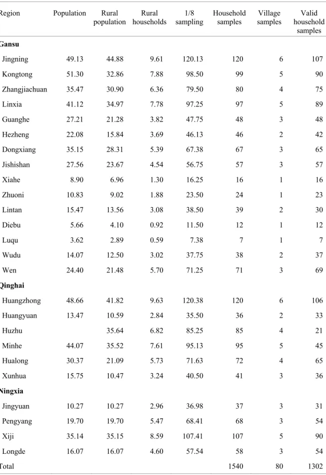
Firstly 25 extreme poor counties from 3 provinces were chosen as being the study areas. Based on the rural population and rural households of those targeted counties, 73 extreme poor villages were selected as the village samples following a PPS sampling that randomly drawn 20-25 household samples from each village. In total, there are 1302 valid samples by 2 rounds survey from 7 ethnic groups of Hans, Hui, Tibetan, Dongxiang, Baoan, Salar, Tibetan and Tu are included in the survey.

(15)

Table 1.1 Sampling and survey samples

Region Population Rural

population households Rural sampling 1/8 Household samples samples Village household Valid samples Gansu Jingning 49.13 44.88 9.61 120.13 120 6 107 Kongtong 51.30 32.86 7.88 98.50 99 5 90 Zhangjiachuan 35.47 30.90 6.36 79.50 80 4 75 Linxia 41.12 34.97 7.78 97.25 97 5 89 Guanghe 27.21 21.28 3.82 47.75 48 3 48 Hezheng 22.08 15.84 3.69 46.13 46 2 42 Dongxiang 35.15 28.31 5.39 67.38 67 3 65 Jishishan 27.56 23.67 4.54 56.75 57 3 57 Xiahe 8.90 6.96 1.30 16.25 16 1 16 Zhuoni 10.83 9.02 1.88 23.50 24 1 23 Lintan 15.47 13.56 3.08 38.50 39 2 30 Diebu 5.66 4.10 0.92 11.50 12 1 12 Luqu 3.62 2.89 0.59 7.38 7 1 7 Wudu 14.07 12.50 3.02 37.75 38 2 37 Wen 24.40 21.48 5.70 71.25 71 3 69 Qinghai Huangzhong 48.66 41.82 9.63 120.38 120 6 106 Huangyuan 13.47 10.59 2.84 35.50 36 2 33 Huzhu 35.64 6.82 85.25 85 4 21 Minhe 44.07 35.52 7.61 95.13 95 5 45 Hualong 30.37 21.09 5.73 71.63 72 4 65 Xunhua 15.75 10.47 3.24 40.50 41 3 36 Ningxia Jingyuan 10.27 10.27 2.96 36.98 37 3 31 Pengyang 19.70 19.70 5.47 68.41 68 3 54 Xiji 35.14 35.15 8.59 107.41 107 5 90 Longde 16.07 16.07 4.60 57.54 58 3 54 Total 1540 80 1302

Data source: Gansu Development Yearbook 2015, Ningxia Statistical Yearbook 2015, Qinghai Statistical Yearbook 2015 and own survey.

(16)

7

1.5 Structure of the Study

The present research has been divided into seven chapters.

The first chapter covered the background of poverty reduction and poverty studies in China, literature review, research objectives and study areas of the present research. The literature review specially introduced the previous studies on poverty dynamics include the definition and main research patterns of poverty dynamics.

The second chapter is mainly an introduction into the poverty dynamics in northwest China by official statistics data.

The third and fourth chapter are the main findings of the present research in responses of the research objectives. Using a regional survey dataset, Chapter 3 estimated the effect of farm diversification that is considered as an important behaviour in agricultural production on poverty reduction and poverty dynamics in a short-term. Chapter 4 similarly estimated the effect of rural labour migration on poverty reduction and poverty dynamics in a short-term. According to the results of these two chapters, the appropriate poverty reduction policy suggestions were proposed.

The fifth chapter estimated the effect of social capital, being considered as an important individual indicator to rural household welfare, on poverty reduction and poverty dynamics in a short-term. And the sixth chapter is introduced the household-level poverty targeting methods and checked the method efficiency in different sorts of poverty reduction projects under different poverty lines.

The whole work is concluded in the seventh chapter. This chapter includes the conclusion, discussion and further recommendations made based on results.

(17)

CHAPTER 2

POVERTY DYNAMICS IN NORTHWEST CHINA: AN OVERVIEW

2.1 Northwest China

Fig. 2.1 Map of Northwest of China

Northwest China is comprised of three provinces of Gansu, Qinghai and Shaanxi and two autonomous regions of Xinjiang and Ningxia. The land area of northwest China, covering above 14% terrestrial land area of China, is highly varied and includes large stretches of arid desert and wasteland, fertile oases, grassy plateaus, and high mountain ranges.

The overall population of northwest China is about 100 million that shares 7.3% of the total population of China. A large percentage of the population belongs to ethnic minority groups of Hui, Uyghurs, Kazak, Kirgiz, Mongols and Tibetan, and northwest China has been recognized as a typical ethnic-minority area.

(18)

9

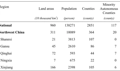
Table 2.1 Basic statistics of Northwest China in 2016

Region _{Land areas} _Population _Counties _AutonomousMinority Counties

(10 thousand km2₎ _(person) _(county) _(county)

National 960 138271 2851 117 Northwest China 311 10089 364 20 Shannxi 21 3813 107 0 Gansu 45 2610 86 7 Qinghai 72 593 44 7 Ningxia 7 675 22 0 Xinjiang 166 2398 105 6

Data source: China Statistical Yearbook 2017.

The economy of northwest China shared a low percentage of the whole China. Both the per capita GDP (41989 yuan) and government revenue (455 billion yuan) of northwest China are lower than the national average level.

Table 2.2 Basic statistics of Northwest China in 2016

Region Per capita GDP Government revenue Total investment Household consumption level

(yuan) (billion yuan) (billion yuan) (yuan)

National 53680 15960 60647 21285 Northwest China 41989 455 4810 16062 Shannxi 51015 183 2083 16657 Gansu 27643 79 966 13086 Qinghai 43531 24 353 16751 Ningxia 47194 39 379 18570 Xinjiang 40564 130 1029 15247

(19)

Fig2.2 China’s Rural Poverty Distribution

Source: Liu, et al. (2016) Regional Differentiation Characteristics of Rural Poverty and Targeted Poverty Alleviation Strategy in China

2.2 Poverty Dynamics in Northwest China

Northwest China has been considered as one of the poorest regions of China and faces an enormous challenge to promote poverty reduction (Zhou et.al, 2018). Using the Chinese government poverty line of 2300 yuan (about $334) in annual income, it was counted by official statistics that about 7 million people in northwest China were still living under poverty by the end of 2016, that shared 16.05% of the total poor population of China. The poverty rate of northwest China stands twice higher than the national level (NBS, 2017).

From a dynamic statistical perspective, rural poor population in northwest China fell from 14.94 million in 2012 to 6.96 million in 2016, that the total population living under poverty

(20)

11 has reduced by 53.41% within five years. Compared within provinces, Gansu, Xinjiang and Shaanxi contributes a large percentage of the poor population.

Table 2.2 Rural poor population in Northwest China 2012-2016

Region Rural poor population (10 thousand persons) 2012 2013 2014 2015 2016 National 9899 8249 7017 5575 4335 Northwest China 1494 1242 1076 872 696 Shannxi 483 410 350 288 226 Gansu 596 496 417 325 262 Qinghai 82 63 52 42 31 Ningxia 60 51 45 37 30 Xinjiang 273 222 212 180 147

Data source: Poverty Monitoring Report of Rural China 2016 and 2017.

The poverty rate in northwest China decreased from 21.4% in 2012 to 9.8% in 2016, however it is still higher than the national level (4.5%) even though the poverty reduction speed was in accordance with the national level.

Table 2.3 Rural poverty rate in Northwest China 2012-2016

Region Rural poverty rate (%)

2012 2013 2014 2015 2016 National 10.2 8.5 7.2 5.7 4.5 Northwest China 21.4 17.5 15.2 12.4 9.8 Shannxi 17.5 15.1 13.0 10.7 8.4 Gansu 28.5 23.8 20.1 15.7 12.6 Qinghai 21.6 16.4 13.4 10.9 8.1 Ningxia 14.2 12.5 10.8 8.9 7.1 Xinjiang 25.4 19.8 18.6 15.8 12.8

(21)

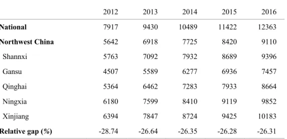
Considering from income and expenditure of rural household, by the end of 2016, per capita net income of rural household in northwest China was going to 9110 yuan while it’s 5642 yuan in 2012, that increased 61.47% within five years. However, the relative gap of per capita net income between northwest China and the national average level almost did not change by about -26%. It is similarly that per capita expenditure of rural household showed an obvious change between 2012 and 2016, however the relative gap to the national average level increased from 2014 on the contrary.

Table 2.4 Poverty dynamics in Northwest China: per capita income 2012-2016

Region Per Capita Income of Rural Households (yuan) 2012 2013 2014 2015 2016 National 7917 9430 10489 11422 12363 Northwest China 5642 6918 7725 8420 9110 Shannxi 5763 7092 7932 8689 9396 Gansu 4507 5589 6277 6936 7457 Qinghai 5364 6462 7283 7933 8664 Ningxia 6180 7599 8410 9119 9852 Xinjiang 6394 7847 8724 9425 10183 Relative gap (%) -28.74 -26.64 -26.35 -26.28 -26.31

Data source: Poverty Monitoring Report of Rural China 2016 and 2017.

Table 2.5 Poverty dynamics in Northwest China: per capita expenditure 2012-2016

Region Per Capita Expenditure of Rural Households (yuan) 2012 2013 2014 2015 2016 National 5908 7485 8383 9223 10130 Northwest China 5050 6698 7335 7882 8538 Shannxi 5115 6488 7252 7901 8568 Gansu 4146 5654 6148 6830 7487 Qinghai 5339 7506 8235 8566 9222 Ningxia 5351 6740 7676 8415 9138 Xinjiang 5301 7103 7365 7698 8277 Relative gap (%) -14.52 -10.51 -12.50 -14.54 -15.71

(22)

13 CHAPTER 3

THE EFFECT OF FARM DIVERSIFICATION ON POVERTY

REDUCTION: EVIDENCE FROM NORTHWEST CHINA

3.1 Introduction

Farm diversification, including multiple cropping, livestock production, rural tourists and family small business has emerged as an equally important alternative to attain the objectives of employment generation, income improvement, and sustainability. It occurs in particularly to promote the local agriculture development and build farmer’s capacity so that more and more serious challenge of returning poverty and livelihood vulnerability (Borm ley and Chavas, 1989; Zhang, 2000; Chen and Li, 2009; Li et al., 2013; Umar I.S. et al., 2015).

Several recent pieces of research recognized that rural household’s farm diversification can raise production efficiency, smoothen risks, improve income and even widen agricultural development space (Xiang and Han, 2005; Chen, 2007; Luo and Deng, 2011; Weng et al., 2017). As to the determinates of rural household’s participation in farm diversification, the previous literature suggested it is impacted by both household capital and agricultural technology extension and policy support (Wang, H. Thomas and G. Thomas, 2007; Chen, 2007; Hao, Li and Xin, 2010; Weng et al., 2017). Some papers considered that farm diversification comes from the seasonal characteristic of agriculture but not the individual differences (Fu and Zhu, 2008; Chao and Huang, 2014). Even so, these researches included rural-to-urban labour migration and family small business, which cannot explain the determinants of local farm diversification and its effects clearly.

Other literature however, presented a different view that the effect of farm diversification on improving the total income of the household and reducing poverty is limited and contractionary (Li and Ye, 2009; Zhu, Hu and Xu, 2014; Xu and Li, 2017). It is because rural household prefers to small-scale investment that usually can’t make a significant contribution to income improvement on one hand. And on another hand of that, farm diversification relies heavily on the support of government which can’t target the poor household (Yang et.al., 2019). Moreover, it might even make rural household fall into a

(23)

low-professional equilibrium trap because the farm diversification may lead to a low income and capital accumulation (Wen and Zhao, 2002; Liu, 2009).

Based on this, this study tries to examine the effects of farm diversification on poverty reduction and poverty dynamics in extremely poor areas from a microcosmic view of household behaviour. Farm diversification here is explained as local agricultural production in different types but it does not include rural-to-urban migration and rural family small business irrelevances to the agricultural sector. Using the regional survey data, this study firstly estimates the effects of farm diversification on improving per capita net income of rural household and poverty by a regression model. Following it, it estimates the effects of farm diversification on poverty dynamics, that was described as the transformation of poverty and non-poverty from 2014 to 2016.

3.2 Data and Variables

This study used the data from own survey conducted at both community and household level collected in 2017 and 2018. We firstly chose 25 extremely poor counties in Gansu Province, Qinghai Province and Ningxia Autonomous Region. Based on the rural population and rural households of those targeted counties, we selected 80 extreme poor villages as the village samples follow a PPS sampling that randomly drawn 20-25 household samples from each village. In total, there are 1302 valid samples from 7 ethnic groups of Hans, Hui, Tibetan, Dongxiang, Baoan, Salar, Tibetan and Tu are included in the survey. Most of the survey villages are in the “poverty-stricken areas” named by National Program for Rural Poverty Alleviation (2001-2010) due to their low income and consumption, less social welfare and insurance, fragile environment, and frequent natural disasters, and their average poverty rate are much worse than the official statistics.

Table 3.1 and Table 3.2 presents the summary statistics for the dependent variables of per capita net income and poverty status in 2014 and 2016. The average per capita net income of the rural household is 4141.64 yuan in 2014 and 4337.31 yuan in 2016. The per capita net income of the household with doing additional farm activities comes to 4722.30 yuan in 2014 and 5101.22 yuan in 2016, which are apparently higher than that of the household without doing any additional farm activities (3961.72 yuan in 2014 and 4044.24 yuan in 2016).

(24)

15

Table 3.1 Summary statistics: Per capita net income in 2014 and 2016

Variables 2014 2016

Mean Std. dev. Mean Std. dev.

All households 4141.64 3341.47 4337.31 3657.06

Farm diversification

Household with additional farming 4722.30 3029.23 5101.22 3359.19 Household without additional farming 3961.72 3133.40 4044.24 3442.77 Data source: Author’s survey

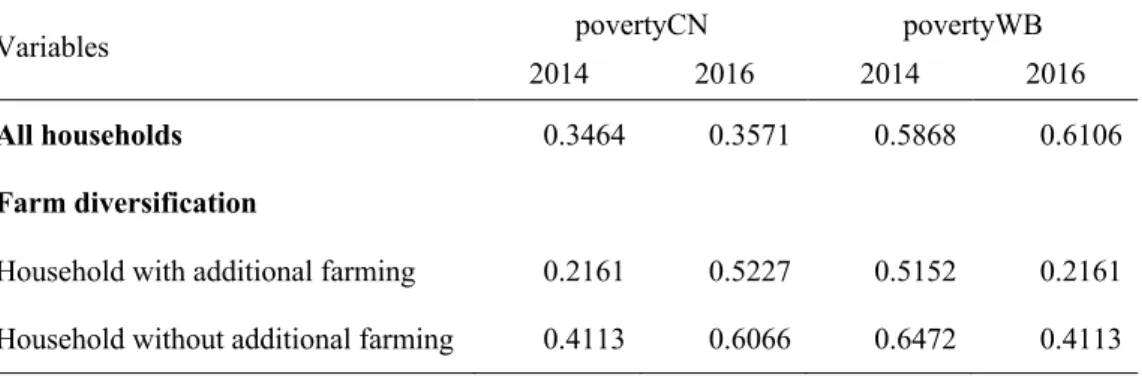
Table 3.2 Summary statistics: Poverty by sorts in 2014 and 2016

Variables povertyCN povertyWB 2014 2016 2014 2016

All households 0.3464 0.3571 0.5868 0.6106

Farm diversification

Household with additional farming 0.2161 0.5227 0.5152 0.2161 Household without additional farming 0.4113 0.6066 0.6472 0.4113 Data source: Author’s survey

Table 3.3 Summary statistics: Poverty dynamics in 2014-2016

Dependent Variables: Poverty dynamics 2014-2016

Obs Mean Std. dev. Poverty Dynamics

under Chinese government line

Poverty to Non-poverty 451 0.2040 0.4034 Non-poverty to Poverty 851 0.1246 0.3304 Poverty Dynamics

under World Bank line

Poverty to Non-poverty 764 0.1152 0.3195 Non-poverty to Poverty 538 0.2212 0.4154 Data source: Author’s survey

(25)

To see the per capita net income from agriculture sector, the summary statistics show a much more obvious difference between the household with and without doing additional farm activities by 500.02 yuan to 3176.40 yuan in 2014 and 514.58 yuan to 3030.00 yuan in 2016.

Then as to poverty, the summary statistics show that poverty raises from 2014 to 2016 in those extreme poor rural areas. Average poverty dummy under the Chinese government standard is 0.3464 in 2014 and 0.3571 in 2016. Changing to a higher standard by World Bank, the poverty dummy come to 0.5868 in 2014 and 0.6106 in 2016 respectively. Seeing the difference of poverty between the household with and without doing additional farm activities, the former has lower results than the latter under all standard poverty line in both 2014 and 2016.

Table 3.3 presents the summary statistics for the dependent variable of poverty dynamics. Taking the poverty line by Chinese government, there’re totally 92 poor households in 2014 got rid of poverty in 2016 while 106 non-poverty dropped into poverty again. Changing to the poverty line by World Bank, the poverty transformation goes to be 143 and 119 respectively.

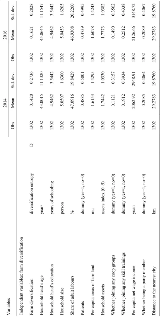
Table 3.4 presents the independent variables. As the main explanatory independent variables, farm diversification here is defined as the dispersion of the total agricultural production expenditure following the definition of diversification entropy by Diao and Lei (2001). The equation of the degree of farm diversification is:

!_" = − % &_'ln (&_')

-'./

where i index household (i=1…i) and j index the production sort (j=1…j); ωj stands for

the percentage of production expenditure of type j in total agricultural production expenditure. Here, we selected 5 sorts of the agricultural production as the crop planting, glasshouse-vegetable and fruits cultivation, livestock breeding, farming business and other. Thus, the value of Di is increased with the household’s production sorts increased while the

value of Di approaches 0 if household only does one type.

According to the summary statistics in Table 3.4, the average of diversification entropy is 0.1420 in 2014 and 0.1621 in 2016.

(26)

17 Ta bl e 3. 4 Sum m ar y st at is ti cs : inde pe nde nt var iabl es Va ri ab le s 2014 2016 Ob s Me an St d. de v. Ob s Me an St d. de v. In de pe nd en t v aria ble s: fa rm di ver si fi cat ion Fa rm di ver si fi cat ion di ver si fi cat ion ent ropy D i 1302 0.1 42 0 0.2 73 6 1302 0.1 62 1 0.2 82 8 Ho us eh ol d he ad ’s a ge year s 1302 43. 0015 11. 1320 1302 45. 0645 11. 1547 Ho us eh ol d he ad ’s e du ca tio n year s of s chool ing 1302 4. 9462 3. 5442 1302 4. 9462 3. 5442 Ho us eh ol d si ze per son 1302 5. 0507 1. 6300 1302 5. 0453 1. 6205 Sha re of a dul t l abour s % 1302 47 .09 16 19 .84 29 1302 46. 9308 20. 2260 Pa tie nt s dum m y (yes = 1, no= 0) 1302 0. 4885 0. 5001 1302 0. 4739 0. 4995 Pe r ca pi ta a re as of f ar m la nd mu 1302 1. 6153 1. 4295 1302 1. 6078 1. 4243 Ho us eh ol d as se ts as set s index (0~ 5) 1302 1. 7442 1. 0330 1302 1. 7773 1. 0382 Wh et he r jo in in g an y co op g ro up s dum m y (yes = 1, no= 0) 1302 0.1 12 1 0.3 15 7 1302 0.1 49 0 0.3 56 2 Wh et he r jo in in g an y sk ill tr ai ni ng s dum m y (yes = 1, no= 0) 1302 0.1 91 2 0.3 93 4 1302 0.2 51 2 0.4 33 8 Pe r ca pi ta ne t w age incom e yuan 1302 2062. 92 2948. 91 1302 2126. 66 3148. 72 Wh et he r be in g a pa rt y m em be r dum m y (yes = 1, no= 0) 1302 0. 2085 0. 4064 1302 0. 2089 0. 4067 Di st an ce to th e ne ar es t c ity km 1302 29. 2783 19. 8760 1302 29. 2783 19. 8760 Da ta s ou rc e: Au th or ’s s ur ve y. No te : 1 m u= 667m 2 or 0. 667 ha

(27)

3.3 Methodology

The method of this study follows a two-step approach to test the effect of farm diversification on income and poverty. We apply an OLS regression model firstly to examine the effect of farm diversification on per capita net income and the following regression equations are given:

ln #_$ = &_'+ &₎*_$ + &₊,_$ + -_$ (1)

Then, the following variables were regressed to estimate the effect of farm diversification on poverty and a Probit estimation is applied to the following equation:

Probit (6_$ = 1) = 9_'+ 9₎*_$ + 9₊,_$ + :_$ (2)

in equations (1) and (2), i index household (i=1,…i); lnY measures log per capita net income of the rural household in yuan and P measures whether the sample household is living under the poverty line, which equals to 1 if poverty and 0 for non-poverty; D stands for farm diversification; H is a vector of the other control variables include household and village characters; µ and ε is the error terms respectively; and β and α are the coefficients to be estimated.

Continuing to analyse the effects of farm diversification on poverty dynamics, we also used the intertemporal Probit model to estimate the probability of the transformation of poverty and non-poverty, and established the empirical models as follows:

Probit (6*_$,A = 1) = B_'+ B₎*_$,AC)+ B₊Δ*_$,A+ 9₊,_$ + E_$ (3)

in equation (3), The symbol t represents the study year of 2016 and t-1 represents the last survey round year of 2014. PD measures the poverty dynamics as the transformation of poverty and non-poverty by reading the definitions of Ye and Zhao (2013). σ is an error term; and δ is the coefficients to be estimated.

(28)

19

3.4 Result analyses

This section presents the main empirical results of the effects of farm diversification on income and poverty.

(1) Estimated effects of farm diversification on income

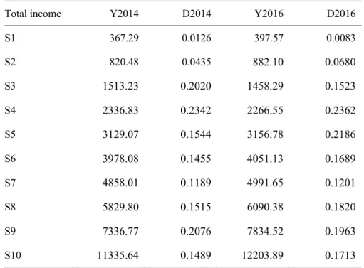
Table 3.5 firstly reports a relationship between per capita net income of the household and farm diversification entropy that seems to be inverse a “wave-type line”. The farm diversification entropy rises at first and goes down later with the increasing of the per capita net income of the household. It is suggested that farm diversification could probably promote rural household’s per capita net income in first stage and specialization on a large-scale production may lead to income improvement in higher stage at an average level. It is matched with the previous study results that the households in different income groups get benefits from specialization or diversification in different stage. Usually, the poor households are specialized in low-yielding activities as the limitation of physical capital and social capital and would be positively impacted by farm diversification. While rich households are specialized in high-yielding activities and likely to benefit as the scale production.

Table 3.5 Farm diversification and total income of the household

Total income Y2014 D2014 Y2016 D2016 S1 367.29 0.0126 397.57 0.0083 S2 820.48 0.0435 882.10 0.0680 S3 1513.23 0.2020 1458.29 0.1523 S4 2336.83 0.2342 2266.55 0.2362 S5 3129.07 0.1544 3156.78 0.2186 S6 3978.08 0.1455 4051.13 0.1689 S7 4858.01 0.1189 4991.65 0.1201 S8 5829.80 0.1515 6090.38 0.1820 S9 7336.77 0.2076 7834.52 0.1963 S10 11335.64 0.1489 12203.89 0.1713 Data source: Author’s survey

(29)

Sequentially, Table 3.6 presents the effect of farm diversification on per capita income of the household by using the predicting outcomes of the model above. Both the coefficients of farm diversification in 2014 and 2016 were found significantly positive as 0.6954 and 0.8655 at 1% level.

In terms of the control variables, compared with the omitted baseline group of the illiterate or semi-illiterate, the middle school-educated, and other higher level-educated household tends to decrease income. Specifically, the coefficients before the share of higher level-educated households are highly significant in per capita net income of the household, which suggests a highly robust income-improving effect of higher education. The share of adult labour tends to increase the per capita net income of the household, whereas the family size tends to decrease the per capita net income. Here, this is due to whether agricultural production or rural labour migrant work is labour intensive. Same as the result in Chapter 3, the household having a patient is significantly negative while farmland areas, household assets are significantly positive in increasing per capita net income of the household at a high level in both 2014 and 2016.

Particularly targeting to analyse the farm diversification, the control variables of joining coop-organization and skill training is chosen and found significant in increasing per capita net income of the household. The control variable of wage income is recognized as one important factor that impacts income improvements. The result suggests that wage income tends to increase per capita net income of the household, as the estimated coefficient is highly significant.

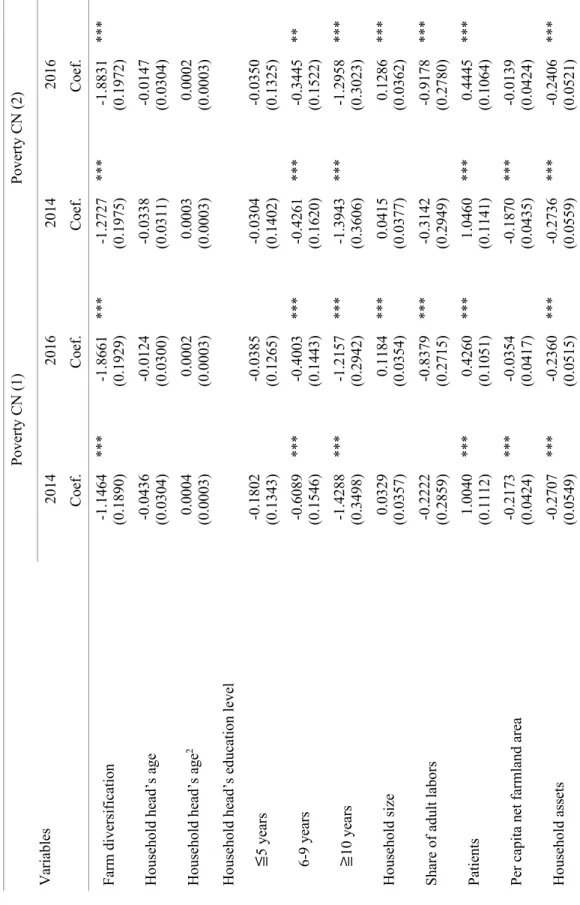
(2) Estimated effects of farm diversification on poverty

Table 3.7 shows that farm diversification has significant effects on poverty reduction in 2014 and 2016 respectively as the estimated coefficient is highly significant at the level of 1%. The estimated coefficient in 2016 highly increases than that in 2014, that suggests a significant promoting effect between the two adjacent periods. We understand that farm diversification could be helpful for reducing poverty in the short term, by supported additional agricultural production projects and following plantation that has been proved with a profit by other village members, however the successional level and intertemporal effects cannot be found from the result. As the

(30)

21 the omitted baseline group of the illiterate or semi-illiterate, the middle school-educated and other higher level-educated household can decrease the probability of falling into poverty. Family size and the share of adult labour are not significant in reducing the household’s poverty but contrary to 2016. A positive trend is observed in variables “farmland areas” and “household assets” and “being a Party member” while a negative trend in the control variable of “having a patient member”, that is matched the results in Table 3.7.

Specially for the analysing to agricultural production, the control variables of “joining skill training” and “wage income” have significant positive effects on poverty reduction in both 2014 and 2016. It could be explained that a skill training toward the agricultural production, especially to the field of additional agricultural production usually with a high additional value, tends to be more likely to make the household achieve an effective income improvement. And the variables of “wage income” also explain part of the income sources and the contributed percentage to the poverty gap.

But, the variable of “joining a coop organization”, that to be interestingly found, shows a different estimated effect in two adjacent periods and does not show significance in 2016. As the interview to rural household, joining a rural technological cooperative or agricultural products sales cooperative was further popularized in 2016 since the local governments promoted the targeting poverty reduction. However, the direct benefit from joining a cooperative organization turned to be more averaged at a low-level, so that bedimmed the estimated effects.

(3) Comparison among ethnic groups

The results of difference effect between ethnic minority groups and Han are presented in Table 3.6 and Table 3.7. It suggests that ethnic group of Hui, Dongxiang and Baoan have a negative gap in effects on income and poverty reduction by comparing with Han in 2014 while the significance is shown only on side of the ethnic group of Dongxiang and Tibetan in 2016.

It is noted that compared with the omitted baseline group of Hans, ethnic group of Hui, Dongxiang, Baoan and Tibetan have a lower trendy to increase per capita net income and reduce the poverty rate in 2014. Ethnic group Hui, Dongxiang and Baoan have a negative gap in effects on income and poverty reduction by comparing with Han in 2014 since the different rural labour migrant work decision and income gap.

(31)

In 2016 however, the difference to Hui turns opposite that comparing with Han, Huis tend to achieve more per capita income and reduce the probability of falling into poverty. It’s quite possibly because of the contribution of the effective poverty reduction in Ningxia Autonomous Region, in which most of the samples are Huis.

There are no significant results seen from the ethnic groups of Salar, Tibetan and Tu. This could be because the Tibetans and Tus in this sample set are from different communities and environments leading to inconsistent results.

(4) Estimated effects of farm diversification on poverty dynamics

A significantly positive coefficient of the change of farm diversification on the transformation of poverty to non-poverty in Table 3.8 indicates that an increasing entropy of farm diversification of the household tends to promote the transformation of poverty to non-poverty.

While as to the estimated effect of farm diversification on the transformation of non-poverty to non-poverty, the change of farm diversification as well as the estimated farm diversification entropy in 2014 have a significantly negative impact on the transformation at a 1% level.

Besides, the estimated result also suggested that both the change of patients and patient number of the household in 2014 have significant effects on transformation of poverty to non-poverty respectively. We understand that the expenditure of both money and time for the patient member would seriously affect the family welfare. The per capita net farmland areas in 2014 and household assets in 2014 have positive effects on transformation of poverty to non-poverty as the estimated coefficient is highly significant. It is probably because that the accumulation of the household assets needs taking a certain amount of time so that rural household’s original assets and resources have a strong effect on maintaining family welfare.

(32)

23 Ta bl e 3. 6 Th e ef fe ct s of fa rm d iv er sific atio n on incom e, O LS Va ri ab le s Lo g (P er c ap ita n et in co m e) ( 1) Lo g (P er c ap ita n et in co m e) ( 2) 2014 2016 2014 2016 Co ef . Co ef . Co ef . Co ef . Fa rm di ver si fi cat ion 0. 6954 (0 .0 74 8) *** 0. 8655 (0 .0 75 0) *** 0. 7442 (0 .0 75 5) *** 0. 8775 (0 .0 76 0) *** Ho us eh ol d he ad ’s a ge 0. 0043 (0 .0 10 9) 0. 0070 (0 .0 11 5) 0. 0014 (0 .0 10 9) 0. 0072 (0 .0 11 5) Ho us eh ol d he ad ’s a ge 2 -0. 0001 (0 .0 00 1) -0. 0001 (0 .0 00 1) -0. 0000 (0 .0 00 1) -0. 0001 (0 .0 00 1) Ho us eh ol d he ad ’s e du ca tio n le ve l ≦ 5 year s 0. 0758 (0 .0 48 5) 0. 0058 (0 .0 48 6) 0. 0386 (0 .0 50 3) 0. 0058 (0 .0 50 6) 6-9 year s 0. 2055 (0 .0 55 3) *** 0. 1284 (0 .0 55 2) ** 0. 1548 (0 .0 57 6) *** 0. 1167 (0 .0 57 9) ** ≧ 10 year s 0. 6311 (0 .1 09 3) *** 0. 6274 (0 .1 09 4) *** 0. 5629 (0 .1 09 7) *** 0. 6119 (0 .1 10 5) *** Ho us eh ol d si ze -0. 0128 (0 .0 12 5) -0. 0474 (0 .0 12 8) *** -0. 0164 (0 .0 12 5) -0. 0516 (0 .0 12 8) *** Sha re of a dul t l abor s 0. 1767 (0 .1 01 3) * 0. 4226 (0 .0 99 6) *** 0. 1960 (0 .1 00 9) * 0. 4440 (0 .0 99 8) *** Pa tie nt s -0. 4530 (0 .0 41 0) *** -0. 2484 (0 .0 40 5) *** -0. 4650 (0 .0 40 8) *** -0. 2568 (0 .0 40 5) *** Pe r ca pi ta ne t f ar m la nd ar ea 0. 0943 (0 .0 14 4) *** 0. 0332 (0 .0 14 5) ** 0. 0860 (0 .0 14 5) *** 0. 0282 (0 .0 14 7) * Ho us eh ol d as se ts 0. 1067 (0 .0 19 4) *** 0. 1046 (0 .0 19 3) *** 0. 1060 (0 .0 19 3) *** 0. 1036 (0 .0 19 3) ***

(33)

24 Wh et he r jo in in g an y co op g ro up s 0. 2314 (0 .0 68 6) *** 0. 1262 (0 .0 60 8) ** 0. 2091 (0 .0 68 7) *** 0. 1361 (0 .0 61 7) ** Wh et he r jo in in g an y sk ill tr ai ni ng s 0. 1607 (0 .0 19 4) *** 0. 1162 (0 .0 52 8) ** 0. 1447 (0 .0 55 4) *** 0. 1069 (0 .0 53 2) ** Pe r ca pi ta ne t w age inc om e 0. 0002 (7 .1 7e -06) *** 0. 0002 (6 .5 5e -06) *** 0. 0002 (7 .2 5e -06) *** 0. 0002 (6 .6 3e -06) *** Pa rt y me mb er sh ip 0. 1810 (0 .0 48 1) *** 0. 1911 (0 .0 48 2) *** 0. 1806 (0 .0 48 1) *** 0. 1922 (0 .0 48 5) *** Di st an ce to th e ne ar es t c ity 0. 0004 (0 .0 01 0) 0. 0004 (0 .0 01 0) 0. 0011 (0 .0 01 1) 0. 0006 (0 .0 01 1) Et hn ic g ro up s Hu i -0. 1104 (0 .0 47 4) ** 0. 0184 (0 .0 48 4) Do ng xi an g -0. 1193 (0 .0 71 7) * -0. 0235 (0 .0 72 4) Ba oa n -0. 5101 (0 .1 34 7) *** -0. 2543 (0 .1 35 9) * Sa la r 0. 1122 (0 .1 07 4) 0. 1865 (0 .1 08 2) Ti ba te n -0. 2438 (0 .0 67 8) *** -0. 1322 (0 .0 68 0) * Tu -0. 2941 (0 .2 25 0) -0. 2956 (0 .2 26 8) Co ns ta nt 7. 0237 (0 .2 66 3) *** 7. 3420 (0 .2 88 8) *** 7. 2438 (0 .2 71 9) *** 7. 3852 (0 .2 96 0) *** Da ta s ou rc e: Au th or ’s s ur ve y No te : ***, **, * m eans s igni fi cant at 1% , 5% , 10% pr obabi lit y level r es pect ivel y.

(34)

25 Ta bl e 3. 7 Th e ef fe ct s of fa rm d iv er sific atio n on povert y, Pr ob it Va ri ab le s Pove rt y C N (1 ) Wo rl d B an k Po ve rt y L in e Pove rt y C N ( 2) 2014 2016 2014 2016 Co ef . Co ef . Co ef . Co ef . Fa rm di ve rs if ic at ion -1. 1464 (0 .1 89 0) *** -1. 8661 (0 .1 92 9) *** -1. 2727 (0 .1 97 5) *** -1. 8831 (0 .1 97 2) *** Ho us eh ol d he ad ’s a ge -0. 0436 (0 .0 30 4) -0. 0124 (0 .0 30 0) -0. 0338 (0 .0 31 1) -0. 0147 (0 .0 30 4) Ho us eh ol d he ad ’s a ge 2 0. 0004 (0 .0 00 3) 0. 0002 (0 .0 00 3) 0. 0003 (0 .0 00 3) 0. 0002 (0 .0 00 3) Ho us eh ol d he ad ’s e du ca tio n le ve l ≦ 5 year s -0. 1802 (0 .1 34 3) -0. 0385 (0 .1 26 5) -0. 0304 (0 .1 40 2) -0. 0350 (0 .1 32 5) 6-9 year s -0. 6089 (0 .1 54 6) *** -0. 4003 (0 .1 44 3) *** -0. 4261 (0 .1 62 0) *** -0. 3445 (0 .1 52 2) ** ≧ 10 year s -1. 4288 (0 .3 49 8) *** -1. 2157 (0 .2 94 2) *** -1. 3943 (0 .3 60 6) *** -1. 2958 (0 .3 02 3) *** Ho us eh ol d si ze 0. 0329 (0 .0 35 7) 0. 1184 (0 .0 35 4) *** 0. 0415 (0 .0 37 7) 0. 1286 (0 .0 36 2) *** Sha re of a dul t l abor s -0. 2222 (0 .2 85 9) -0. 8379 (0 .2 71 5) *** -0. 3142 (0 .2 94 9) -0. 9178 (0 .2 78 0) *** Pa tie nt s 1. 0040 (0 .1 11 2) *** 0. 4260 (0 .1 05 1) *** 1. 0460 (0 .1 14 1) *** 0. 4445 (0 .1 06 4) *** Pe r ca pi ta ne t f ar m la nd ar ea -0. 2173 (0 .0 42 4) *** -0. 0354 (0 .0 41 7) -0. 1870 (0 .0 43 5) *** -0. 0139 (0 .0 42 4) Ho us eh ol d as se ts -0. 2707 (0 .0 54 9) *** -0. 2360 (0 .0 51 5) *** -0. 2736 (0 .0 55 9) *** -0. 2406 (0 .0 52 1) ***

(35)

26 Wh et he r jo in in g an y co op g ro up s -0. 4787 (0 .1 71 6) *** -0. 1831 (0 .1 44 4) -0. 4427 (0 .1 75 6) ** -0. 2040 (0 .1 49 4) Wh et he r jo in in g an y sk ill tr ai ni ng s -0. 3089 (0 .1 43 0) ** -0. 2723 (0 .1 33 5) ** -0. 2472 (0 .1 47 3) * -0. 2276 (0 .1 36 0) * Pe r ca pi ta ne t w age inc om e -0. 0009 (0 .0 00 1) *** -0. 0008 (0 .0 00 1) *** -0. 0010 (0 .0 00 1) *** -0. 0009 (0 .0 00 1) *** Pa rt y m em be rs hi p -0. 3654 (0 .1 28 1) *** -0. 4878 (0 .1 26 8) *** -0. 3256 (0 .1 30 6) ** -0. 4780 (0 .1 29 0) *** Di st an ce to th e ne ar es t c ity 0. 0027 (0 .0 02 6) 0. 0030 (0 .0 02 6) 0. 0029 (0 .0 03 0) 0. 0013 (0 .0 03 0) Et hn ic g ro up s Hu i 0. 3760 (0 .1 30 0) *** -0. 1389 (0 .1 26 4) Do ng xi an g 0. 9669 (0 .2 39 9) *** 0. 4130 (0 .2 04 9) ** Ba oa n 1. 0489 (0 .3 37 9) *** 0. 5151 (0 .3 26 0) Sa la r -0. 2880 (0 .3 91 5) -0. 6208 (0 .3 76 0) * Ti ba te n 0. 4721 (0 .1 88 4) ** 0. 2023 (0 .1 80 5) Tu 0. 6312 (0 .6 09 3) 0. 7908 (0 .6 24 5) Co ns ta nt 1. 9133 (0 .7 54 4) *** 0. 8969 (0 .7 57 3) *** 1. 0833 (0 .7 84 4) *** 0. 7073 (0 .7 81 8) *** Da ta s ou rc e: Au th or ’s s ur ve y No te : ***, **, * m eans s igni fi cant at 1% , 5% , 10% pr obabi lit y level r es pect ivel y.

(36)

27

Table 3.8 The effects of farm diversification on poverty dynamics, Probit

Variables

Poverty to

Non-poverty Non-poverty to Poverty Coef. Coef.

Change of Farm diversification _(0.4997)1.4992 *** _(0.5140)-3.0142 *** Farm diversification 2014 _(0.4037)1.0846 *** _(0.3560)-1.9585 *** Change of Family size _(2.1989)-0.2075 _(1.0154)-0.7560 Family size 2014 _(0.0714)-0.1489 ** _(0.0554)0.1441 ** Change of the share of adult labour _(4.5876)4.0576 _(3.0014)-5.7905 ** Share of adult labour 2014 _(0.5481)0.8124 _(0.4199)-0.9620 ** Change of patients _(0.5353)-0.5928 _(0.4000)0.8272 *** Patients 2014 _(0.1716)0.0424 _(0.1198)0.1172 Change of per capita net farmland areas _(0.1296)-0.1514 _(0.5835)0.1014 Per capita net farmland areas 2014 _(0.1014)0.1296 _(0.0458)0.2142 Change of household assets _(0.5147)0.1297 _(0.3470)-0.0871 Household assets 2014 _(0.1117)-0.0079 _(0.0796)-0.2716 Change of wage income _(0.0000)0.0002 *** _(0.0000)-0.0002 *** Wang income 2014 _(0.000)0.0000 *** _(0.0000)-0.0001 *** Change of agricultural expenditure _(0.0004)0.0018 *** _(0.0001)-0.0000 Agricultural expenditure 2014 _(0.0004)0.0006 * _(0.0001)-0.0001 Constant _(0.5774)-1.8035 *** _(0.4284)-0.5934 Data source: Author’s survey

(37)

3.5 Conclusion and Discussion

Drawing upon a regional household survey data in 2014 and 2016, the present study analysed rural household’s participation in farm diversification, such as doing fruit-vegetable cultivation, livestock farming and family small business respectively and its effect on poverty reduction and transformation of poverty status in a short-term. The results suggest that diversiform farming of the rural household significantly improved the per capita net income and reduced their poverty, as well as the significantly positive effect on transformation of poverty to non-poverty has been found. However, it did not show a result that the details of which kind of agricultural production combination would be best for increasing income and reducing poverty.

A main policy implication of this study is that local government or NGO poverty reduction projects should adopt targeted policies to promote farm diversification with supporting basic agricultural tools or transportation, and agricultural corporatization movements as to encourage more participates in farm diversification. To understand the poverty reduction policies widely, the promotion of farmer entrepreneurship in rural areas, such as the support for setting up cooperation organizations and skill training, agricultural extension should be put more attentions.

(38)

29 CHAPTER 4

THE EFFECT OF RURAL LABOUR MIGRATION ON POVERTY

REDUCTION: EVIDENCE FROM NORTHWEST CHINA

4.1 Introduction

Since the mid-1980s, China’s economic growth has been driven primarily by rapid industrialization and urbanization in which rural labour is steadily leaving agriculture for higher returns in the non-agricultural sector (Du, Park and Wang, 2005). In the past 20 years, the number of rural-to-urban migrant workers in China increased from 79 million to over 281 million until 2016 (NBS, 2016), that represents one of the biggest migrations in human history (Roberts, 2007) and greatly improved their lives.

Rural labour migration has been well known as a vital way to promote employment, improve income and reduce poverty in rural China (World Bank, 2007; Zhu and Luo, 2010). Researches estimated that rural labour migration contributed to 16-21% of China’s total GDP growth (World Bank,1997; Cai and Wang, 1999; Yao, 2010). The increase in rural labour migrant workers’ income was higher than others by an average of 24% (Yi, 2016; Long and Wang, 2016). Especially for the rural households in less developed regions, labour becomes their most valuable resource for improving income and all family members could enjoy the benefits of the wage income from rural labour migration (Jia, Du and Wang, 2017). As the total income of rural households are significantly increased, savings could be improved and investment capacity in local production enhanced, which was proved helpful to diversify their income source and reduce poverty much more effectively (Ma, 2001; Zhou, 2001; Li, Mao and Zhang, 2008; Zhang, Liu and Fan, 2014). Along the consideration with that, rural labour migration was also recognized playing a functional role in reducing the pressure on demand for land in poor rural areas and contributes to breaking up the vicious cycle of “Poverty-Extensive Cultivation-Ecological

Determinates-Poverty” (Helen Bright etc., 2000; de Brauw and Giles, 2008; Liu, 2015),

(39)

Fig 4.1 Contribution of Rural labour migration to GDP Growth, 2001-2016

Data sources: NBS (2002-2017), NDRC (2002-2017).

In addition to that, several articles suggested the role of rural labour migration in reducing inequality and strengthening stability of poverty reduction (Zhu and Luo, 2010; Cai and Du, 2011; Xue, Gao and Lin, 2014; Jia, Du and Wang, 2016), that would be another sustainable poverty reduction view.

However, between the years 2012-2016, the growth of rural-to-urban labour migrant workers were slowing yearly and some researches pointed out a sceptical attitude on whether rural labour migration still plays an important effect on increasing income and reducing poverty, especially in poverty-stricken areas of middle and western China (Yang, 2012; Pu and Luo, 2015; Zhang, 2017). On one hand of this, the rural labour migrant workers are likely to get fewer job opportunities and lower wages in part because it is becoming less demand for the labour-intensive work with the profound economic and social structure transformation. On another hand, rural labour migrant workers also face the risk of becoming a “new poor class” in urban areas, because the social protection networks have not been unified between rural and urban areas (Wang, 2010; Jia, Du and Wang, 2017). In some cases, researches pointed out the situation that rural labour migrant workers tend to be employed in the industries with high-risk of occupational disease, which would plunge into severe and even life-threatening bouts that could probably increase their risk of falling into poverty (Wang, 2010; Liu et al., 2015).

(40)

31 The overall goal of this study is to examine the effects of rural labour migration on poverty reduction in a dynamic research view in northwest China. To meet this goal, it firstly estimates the effects of rural labour migration on improving per capita net income and poverty of the household by a two-step regression model. Following it, it analyses the effects of rural labour migration on poverty dynamics, that was described as the transformation of poverty and non-poverty in adjacent two periods.

3.2 Data Collection and Variables

This study contains data from own survey conducted at both community and household level collected in 2017 and 2018. We firstly chose 25 extremely poor counties in Gansu Province, Qinghai Province and Ningxia Autonomous Region. Based on the rural population and rural households of those targeted counties, we selected 73 extreme poor villages as the village samples follow a PPS sampling that randomly drawn 20-25 household samples from each village. In total, there are 1302 valid samples from 7 ethnic groups of Hans, Hui, Tibetan, Dongxiang, Baoan, Salar, Tibetan and Tu are included in the survey. Most of the survey villages are in the “poverty-stricken areas” named by National Program for Rural Poverty Alleviation (2001-2010) due to their low income and consumption, less social welfare and insurance, fragile environment and frequent natural disasters, and their average poverty rate are much worse than the official statistics.

Table 4.1and Table 4.2 presents the summary statistics for the dependent variables of income and poverty. Firstly, the average per capita net income of the rural household is 4141.64 yuan in 2014 and 4337.31 yuan in 2016. The per capita net income of the household with rural labour migrant worker comes to 5664.15 yuan in 2014 and 5995.56yuan, which are apparently higher than that of the household without rural labour migrant worker (2992.57 yuan in 2014 and 3129.67 yuan in 2016). From the income structure, we can deduce that migrant work is the main source of income for migrant households as 81.51% of total income while agriculture is the main source of income for non-migrant households as 72.25%.

Then as to poverty, the summary shows that the poverty rate raises from 2014 to 2016 in those extremely poor rural areas. The average poverty dummy under the Chinese government standard is 0.3464 in 2014 and 0.3571 in 2016. Changing to a higher standard by World Bank, the poverty comes to 0.5868 in 2014 and 0.6106 in 2016 respectively.

(41)

Table 4.1 Summary statistics: Per capita net income in 2014 and 2016

Variables 2014 2016

Mean Std. dev. Mean Std. dev. All households 4141.64 3341.47 4337.31 3657.06

Labour migrants

Household with labour migrants 5664.15 2953.39 5995.56 3467.74 Household without labour migrants 2992.57 3154.28 3120.67 3298.29 Data source: Author’s survey

Table 4.2 Summary statistics: Poverty by sorts in 2014 and 2016

Variables povertyCN povertyWB 2014 2016 2014 2016 All households 0.3464 0.3571 0.5868 0.6106

Labour migrants

Household with labour migrants 0.0768 0.1034 0.3500 0.4029 Household without labour migrants 0.5499 0.5433 0.7655 0.7630 Data source: Author’s survey

Table 4.3 Summary statistics: Poverty dynamics in 2014-2016

Dependent Variables: Poverty dynamics 2014-2016

Obs Mean Std. dev. Poverty Dynamics

under Chinese government line

Poverty to Non-poverty 451 0.2040 0.4034 Non-poverty to Poverty 851 0.1246 0.3304 Poverty Dynamics

under World Bank line

Poverty to Non-poverty 764 0.1152 0.3195 Non-poverty to Poverty 538 0.2212 0.4154 Data source: Author’s survey.

(42)

33 Ta bl e 4. 4 Sum m ar y st at is ti cs : Inde pe nde nt var iabl es Va ri ab le s 2014 2016 Ob s Me an St d. de v. Ob s Me an St d. de v. In de pe nd en t v aria ble s: la bo ur mi gr at io n Wh et he r ha vi ng m ig ra nt w or ke r dum m y (yes = 1, no= 0) X i 1302 0. 4301 0. 4952 1302 0. 4232 0. 4943 IV : P erc en ta ge o f m ig ra nts in v illa ge % Z i 1302 42. 0656 19. 6626 1302 41. 4849 18. 4128 Ho us eh ol d he ad ’s a ge year s 1302 43. 0015 11. 1320 1302 45. 0645 11. 1547 Ho us eh ol d he ad ’s e du ca tio n year s of s chool ing 1302 4. 9462 3. 5442 1302 4. 9462 3. 5442 Ho us eh ol d si ze per son 1302 5. 0507 1. 6300 1302 5. 0453 1. 6205 Sha re of a dul t l abour s % 1302 47 .09 16 19 .84 29 1302 46. 9308 20. 2260 Sha re of chi ldr en under 16 year s ol d % 1302 25. 9547 19. 8056 1302 25. 9363 19. 8125 Pa tie nt s dum m y (yes = 1, no= 0) 1302 0. 4885 0. 5001 1302 0. 4739 0. 4995 Pe r ca pi ta a re as of f ar m la nd mu 1302 1. 6153 1. 4295 1302 1. 6078 1. 4243 Ho us eh ol d as se ts as set s index (0~ 5) 1302 1. 7442 1. 0330 1302 1. 7773 1. 0382 Wh et he r be in g a pa rt y m em be r dum m y (yes = 1, no= 0) 1302 0. 2085 0. 4064 1302 0. 2089 0. 4067 Di st an ce to th e ne ar es t c ity km 1302 29. 2783 19. 8760 1302 29. 2783 19. 8760 Da ta s ou rc e: Au th or ’s s ur ve y No te : 1 m u= 667m 2 or 0. 667 ha