Exact WKB
analysis of
the harmonic
oscillator
and its Fourier transform
–An example of interplay between
exact
WKB analysis and Fourier analysis
–Yoshitsugu TAKEI
Research
Institute for
Mathematical Sciences
Kyoto University
Kyoto,
606-8502, JAPAN
(京大数理研 竹井義次)
1
Introduction
Although the exact WKB analysis was successful for the global analysis of solutions of
second-order linear ordinary differential equations with a large parameter, its
general-ization to higher-order equations has not been accomplished yet: The local aspect of
the theory such as the connection formula at a simple turning point is established in a
satisfactory manner (cf. [AKTI]), while the global aspect is not fully understood; the
biggest problem is to give a complete description of the Stokesgeometry (i.e., geometry
of Stokes curves) for higher-order equations, which is, in fact, really difficult due to the
necessity of introducing “new Stokes curves” (cf. [BNR], [AKTI], [AKT2]).
In the case of ordinary differential equations of Laplace type, that is, equations
whose coefficients are all linear functions, the Fourier-Laplace transformation gives us
an integral representation ofsolutions and the so-called “steepest descent method” for
the integral representation provides a useful tool for the determination of new Stokes
curves. (Cf. [T2]. See also [U1], [U2]. Note that this point of view is closely related also
to the theory of hyperasymptotics of integrals ([BH], [H] etc.).) We want to generalize
such an approach via integral representations to equations with arbitrary polynomial
coefficients, since the assumption “of Laplace type” is quite restrictive. In this note, as
a starting point of our trial for the generalization, we discuss the well-known harmonic
2Preliminaries –WKB solutions
&their
Borel
transform
The equation we want to discuss in this note is the harmonic oscillator (1) $P \psi=(\frac{d^{2}}{dx^{2}}-\eta^{2}x2+\eta\lambda)\psi--0$
with a parameter $\lambda$
.
Here and in what follows$\eta$ denotes a large parameter. For (1)
there exist the following formal (asymptotic) solutions called WKB solutions:
(2) $\psi_{\pm}=\frac{1}{\sqrt{S_{\mathrm{o}\mathrm{d}\mathrm{d}}}}\exp(\pm\int^{x}S_{\mathrm{o}\mathrm{d}}\mathrm{d}dx)$ , $S_{\mathrm{o}\mathrm{d}\mathrm{d}}= \eta x-\frac{\lambda}{2x}+\cdots$
In particular, let us denote by$\psi_{\pm}^{\mathrm{t}}$ the WKB solutions normalized in the following
way:
(3) $\psi_{\pm}^{\dagger}$
$=$ $\frac{1}{\sqrt{S_{\mathrm{o}\mathrm{d}\mathrm{d}}}}(\eta^{1/2}X)\mp\lambda/2\exp\pm(\eta\frac{x^{2}}{2}+I_{\infty}^{x}(s_{\mathrm{o}\mathrm{d}\mathrm{d}}-\eta X+\frac{\lambda}{2x})dx)$
$=$ $e^{\pm\eta x^{2}/}2 \sum_{n=0}^{\infty}\frac{\psi_{\pm,n}}{X^{2n+(1}\pm\lambda)/2}\eta^{-}(\frac{1}{2}\pm\frac{\lambda}{4}+n)$,
where $\psi_{\pm,n}$ are constants independent of$x$ and $\eta$.
As is well-known, WKB solutions does not converge. In theexact WKB analysis, to
give an analytic meaning to them, we employ the Borel resummation technique. That
is, we regard the Borel sum
(4) $\Psi_{\pm}^{\dagger}=\int_{\mp/2}^{\infty}x^{2}\exp(-\eta y)\psi\uparrow\pm,B(_{X}, y)dy$
as an analytic substitute of them. (In this note a formal series (WKB solution) is
written by a small letter and its Borel sum is denoted by the corresponding capital
letter.) Here the path of integration is assumed to be parallel to the positive real axis
and $\psi_{\pm,B}^{\uparrow}(x, y)$ denotes the Borel transform of$\psi_{\pm}^{\uparrow}$ which is, by definition,
(5) $\psi_{\pm,B}\uparrow(X, y)=\sum^{\infty}n=0\frac{\psi_{\pm,n}}{X^{2n+()/\mathrm{r}(}1\pm\lambda 2\frac{1}{2}\pm\frac{\lambda}{4}+n)}(y\pm\frac{x^{2}}{2})-\frac{1}{2}\pm\frac{\lambda}{4}+n$
The explicit form of$\psi_{\pm,B}^{\uparrow}(X, y)$ is described in terms of Gauss’ hypergeometricfunctions
Lemma 1 Letting $s$ denote $y/x^{2}+1/2$, we have
(6) $\{$
$\psi_{+,B}^{\dagger}(_{X}, y)$ $=$ $\frac{x^{-3/2}}{\Gamma(\frac{1}{2}+\frac{\lambda}{4})}s^{-1/2}+\lambda/4F(\frac{1}{4}+\frac{\lambda}{4}, \frac{3}{4}+\frac{\lambda}{4}, \frac{1}{2}+\frac{\lambda}{4};s)$,
$\psi_{-}^{\uparrow},B(x, y)$ $=$ $\frac{x^{-3/2}}{\Gamma(\frac{1}{2}-\frac{\lambda}{4})}(s-1)^{-}1/2-\lambda/4F(\frac{1}{4}-\frac{\lambda}{4}, \frac{3}{4}-\frac{\lambda}{4}, \frac{1}{2}-\frac{\lambda}{4};1-S)$ .
The expression (6) follows from the following two facts; (i) $\psi_{\pm,B}^{\dagger}(X, y)$ have particular
homogeneity, i.e., $x^{3/2}\psi^{\dagger_{B}}\pm,(x,y)$ are functions of one variable $y/x^{2}$ (or, equivalently, of
$s),$ $(\mathrm{i}\mathrm{i})\psi_{\pm}\dagger_{B(y)},x$, satisfy the Borel transformof equation (1), i.e., $(\partial^{2}/\partial x^{2}-X^{2}\partial 2/\partial y2+$
$\lambda\partial/\partial y)\psi_{\pm}^{\uparrow},B(x, y)=0$
.
For the details of discussion see [Tl, p. 293].Remark 1. In a similar manner we can compute the explicit form of the Borel
trans-form of WKB solutions $\psi_{\pm}\mathrm{t}\mathrm{d}\mathrm{e}\mathrm{f}1/=\eta^{-}\psi 2\dagger\pm$as follows:
(7) $\{$
$\psi_{+}^{\ddagger_{B(x,y)}}$
, $=$ $\frac{x^{-1/2}}{\Gamma(1+\frac{\lambda}{4})}s^{\lambda/4}F(\frac{1}{4}+\frac{\lambda}{4}, \frac{3}{4}+\frac{\lambda}{4},1+\frac{\lambda}{4};\mathrm{q})$,
$\psi_{-,B}^{\ddagger}(_{X}, y)$ $=$ $\frac{x^{-1/2}}{\Gamma(1-\frac{\lambda}{4})}(s-1)^{-}\lambda/4F(\frac{1}{4}-\frac{\lambda}{4}, \frac{3}{4}-\frac{\lambda}{4},1-\frac{\lambda}{4};1-S)$ ,
where $s=y/x^{2}+1/2$
.
This formula will be used in\S 4
and\S 5.
In the case of equation (1) $x=0$ is a unique (double) turning point $\mathrm{a}\mathrm{n}\mathrm{d}\propto sx^{2}=0$
(i.e., the real and imaginary axes) describes the Stokes curves of (1). As a matter
of fact, Lemma 1 implies that Borel sums of $\psi_{\pm}^{\uparrow}$ are well-defined except on the real
and imaginary axes and on each Stokes curve they satisfy the so-called connection
formula (cf. [Tl, Proposition 5]). In the exact WKB theoretictreatmentofthe harmonic
oscillator Borel resummed WKB solutions thus defined play a central role. The main
question we want to discuss in this note is:
QUESTION: How are the Borel resummed WKB solutions transformed by
Fourier-Laplacetransformation with respect to theindependent variable $x$?
3
Steepest descent
method
for the
Fourier
trans-form
The image of the harmonic oscillator (1) under the Fourier-Laplace transformation
(with a large parameter)
is again a harmonic oscillator in the $\xi$-variable
(9) $\hat{P}\hat{\psi}=-(\frac{d^{2}}{d\xi^{2}}-\eta^{2}\xi^{2}-\eta\lambda)\hat{\psi}=0$.
Hence the inverse transformof WKB solutions of (9), in particular,
(10) $\int\exp(\eta_{X}\xi)\hat{\psi}^{\dagger}\pm(\xi, \eta)d\xi=\int\exp(\eta x\xi)\cdot\exp(\pm\eta\frac{\xi^{2}}{2})$
.
(amplitude) $d\xi$,becomes a solution of the harmonic oscillator (1) in the $x$-variable. What we want to
clarify is the relationship between (10) and WKB solutions of (1).
If the amplitude part of the integrand were an ordinary function of $\xi,$ (10) should
be an integral containing a large parameter with the phase function
(11) $\varphi_{\pm}=x\xi\pm\frac{\xi^{2}}{2}$,
and it should be possible to apply the so-called steepest descent method to obtain its
asymptotic expansion for the large parameter $\eta$. Note that, in the case of the “integral
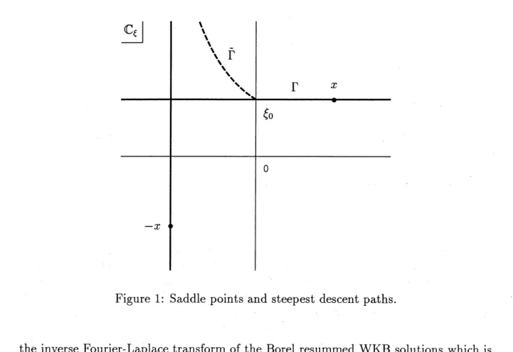
representation” (10), the saddle points of $\varphi\pm \mathrm{a}\mathrm{r}\mathrm{e}\xi=\mp x$ and the steepest (descent)
paths of $\Re\varphi\pm \mathrm{p}\mathrm{a}\mathrm{s}\mathrm{s}\mathrm{i}\mathrm{n}\mathrm{g}$ through $\xi=\mp x$ are given by $\propto s(\xi\pm x)^{2}=0$ respectively (cf.
Figure 1, where the steepest descent paths are drawn by thick lines).
It might thus be expected that the asymptotic expansion of the inverse
Fourier-Laplacetransform of WKB solutions of(9) defined bythe integral (10) along one of such
steepest descent paths should be an asymptotic solution of(1) and hence should become
(possibly a linear combination of) WKB solutions of (1). However, the amplitude part
of (10) is a formal power series of $\eta^{-1}$ and, analytically speaking, it is necessary to
consider its Borel sum instead ofthe formal power series expansion. In the subsequent
sections we discuss the inverse Fourier-Laplace transform of the Borel sum of WKB
solutions of (9) and compare it with theBorel resummed WKB solutions of the original
equation (1).
4
The inverse transform
of the Borel
resummed
WKB solutions
(I) –local theory
In thepreceding sectionwehave observedthatthere aretwosaddlepoints$\xi=\mp x$ of the
phase function$\varphi\pm\cdot$ Since there is no essential difference betweenthem, we only consider
$\xi=x$, which is a saddle point of $\varphi_{-}$, in what follows. For the sake of specification we
also assume that both $\Re x$ and $s^{\infty}x$ are positive (as is shown in Figure 1). Let us denote
Figure 1: Saddle points and steepest descent paths.
the inverse Fourier-Laplace transform of the Borel resummed WKB solutions which is
$\mathrm{d}\mathrm{e}\mathrm{f}\mathrm{i}\dot{\mathrm{n}}$
ed as follows:
(12) $\int_{\Gamma}\exp(\eta_{X}\xi)\hat{\Psi}^{\uparrow(\xi},$ $\eta)d\xi=\int_{\Gamma}\exp(\eta x\xi)(\int_{\xi^{2}/}^{\infty}2\hat{\psi}_{-}\exp(-\eta Z)\uparrow,(\xi B’ z)dZ)d\xi$
.
Employing the following changeof variables ofintegration
(13) $z-x\xi\mapsto y$, $\xi-\xi$,
we find that (12) is equal to
(14) $\int\exp(-\eta y)(\int\hat{\psi}_{-,B}^{\uparrow)}(\xi, y+x\xi)d\xi dy$.
Here let us specify the domain ofintegration of (14). If we introduce new variables
of integration defined by
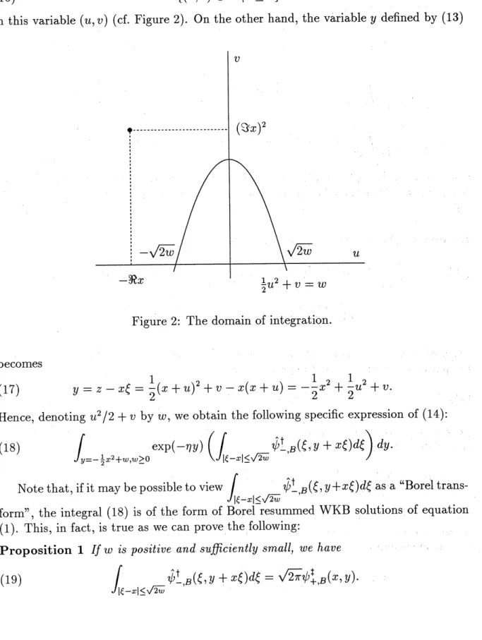
then the domain ofintegration of the original integral (12) is represented by (16) $\{(u, v)\in \mathbb{R}^{2}|v\geq 0\}$
in this variable $(u, v)$ (cf. Figure 2). On the other hand, the variable $y$ defined by (13)
Figure 2: The domain of integration.
becomes
(17) $y=z-x \xi=\frac{1}{2}(x+u)^{2}+v-x(X+u)=-\frac{1}{2}x+\frac{1}{2}u^{2}+v2$.
Hence, denoting $u^{2}/2+v$ by $w$, we obtain the following specific expression of (14):
(18) $\int_{y=-\frac{1}{2}x^{2}}+w,w\geq 0(\exp-\eta y)(\int_{|\xi-x|\leq\sqrt{2w}}\hat{\psi}_{-}\dagger,B(\xi, y+x\xi)d\xi)dy$.
Note that, if it may be possible to view $\int_{|\xi-x}|\leq\sqrt{2w}\hat{\psi}_{-,B}\uparrow(\xi, y+x\xi)d\xi$ asa “Borel
trans-form”, the integral (18) is ofthe form of Borel resummed WKB solutions of equation
(1). This, in fact, is true as we can prove the following:
Proposition 1
If
$w$ is positive and sufficiently small, we haveProof.
It follows from Lemma 1 that the left-hand side of (19) is equal to$\frac{1}{\Gamma(\frac{1}{2}+\frac{\lambda}{4})}\int_{|\xi-x|\leq\sqrt{2w}}\xi-2/3$
$\cross[(s-1)-\frac{1}{2}+\frac{\lambda}{4}F(\frac{1}{4}+\frac{\lambda}{4}, \frac{3}{4}+\frac{\lambda}{4}, \frac{1}{2}+\frac{\lambda}{4};1-S)]|_{s=\frac{y+x\xi}{\epsilon^{2}}+\frac{1}{2}}d\xi$
$=$ $\frac{1}{\Gamma(\frac{1}{2}+\frac{\lambda}{4})}\int_{-\sqrt{2w}}^{\sqrt{2w}}(x+u)^{-2/3}[(-t)^{-\frac{1}{2}+\frac{\lambda}{4}F}(\frac{1}{4}+\frac{\lambda}{4}, \frac{3}{4}+\frac{\lambda}{4}, \frac{1}{2}+\frac{\lambda}{4};t)]|_{t=_{2(+}}u^{2}-2wd\neg xu)u$
$=$ $\frac{x^{-1/2}}{\Gamma(\frac{1}{2}+\frac{\lambda}{4})}\int_{-\sqrt{2a}}^{\sqrt{2a}}(1+u)-2/3[(-t)^{-\frac{1}{2}+\frac{\lambda}{4}F}(\frac{1}{4}+\frac{\lambda}{4}, \frac{3}{4}+\frac{\lambda}{4}, \frac{1}{2}+\frac{\lambda}{4};t)]|t=\frac{u^{2}-2a}{2(1+u)}ud$ ,
where $a=w/x^{2}=y/x^{2}+1/2$. (We have used the scaling $u\mapsto xu$ in obtaining the
last formula.) Then the relation (19) is an immediate consequence of (7) and Lemma 2
below. Q.E.D.
Lemma 2 When $a>0$ is sufficiently small,
(20) $\int_{-\sqrt{2a}}^{\sqrt{2a}}(1+u)-2/3[(-t)^{-\frac{1}{2}+}\frac{\lambda}{4}F(\frac{1}{4}+\frac{\lambda}{4}, \frac{3}{4}+\frac{\lambda}{4}, \frac{1}{2}+\frac{\lambda}{4};t)]|_{t=_{2(1}}u\mp^{2a}2-u)du$
$= \sqrt{2\pi}\frac{\Gamma(\frac{1}{2}+\frac{\lambda}{4})}{\Gamma(1+\frac{\lambda}{4})}a^{\frac{\lambda}{4}}F(\frac{1}{4}+\frac{\lambda}{4}, \frac{3}{4}+\frac{\lambda}{4},1+\frac{\lambda}{4};a)$
.
Proof of
Lemma 2. Let $\alpha,$ $\beta$ and$\gamma$ respectivelydenote $\frac{1}{4}+\frac{\lambda}{4},$ $\frac{3}{4}+\frac{\lambda}{4}$ and $\frac{1}{2}+\frac{\lambda}{4}$
.
Usingthe power series expansion ofhypergeometric functions
(21) $F( \alpha, \beta,\gamma;t)=\sum_{j\geq 0}\frac{(\alpha)_{j}(\beta)_{j}}{(\gamma)_{j}j!}t^{j}$
(where$(\alpha)_{j}=\alpha(\alpha+1)\cdots(\alpha+j-1)=\Gamma(\alpha+j)/\Gamma(\alpha)$etc.), we can rewrite the left-hand
side of (20), denoted by L.H.S. in this proof, as
L.H.S. $= \sum_{j\geq 0}\frac{(\alpha)_{j}(\beta)_{j}}{(\gamma)_{j}j!}(-1)^{j}2^{\frac{1}{2}}-\frac{\lambda}{4}-j\int_{-}^{\sqrt{2a}}\sqrt{2a})(1+u-(\frac{1}{2}+\frac{\lambda}{2}+2j)(2a-u2)^{-\frac{1}{2}}+\frac{\lambda}{4}+jdu$.
Note that the power series expansion (21) is uniformly convergent in the domain of
integration if $a$ is sufficiently small. Furthermore, expanding $(1+u)^{-(1/2+\lambda}/2+2j)$ into
the binomial series (which is also uniformly convergent), we find that
where
$H_{jk}$ $=$ $\int_{-\sqrt{2a}}^{\sqrt{2a}}u^{k}(2a-u^{2})^{-++}\frac{1}{2}\frac{\lambda}{4}jdu$
$=$ $(2a) \frac{\lambda}{4}+j+\frac{k}{2}\int_{-1}^{1}u^{k}(1-u^{2})-\frac{1}{2}+\frac{\lambda}{4}+jdu$
$=$ $\{$
$0$ (when $k$ is odd),
$(2a)^{\frac{\lambda}{4}}+j+ \frac{k}{2}B(\frac{1+k}{2}, \frac{1}{2}+\frac{\lambda}{4}+j)$ (when $k$ is even).
(Here $B(p,$$q)$ denotes the beta function.) We thus obtain
L.H.S. $= \sum_{\iota j,\geq 0}\frac{(\alpha)_{j}(\beta)_{j}}{(\gamma)_{j}j!}\frac{(\frac{1}{2}+\frac{\lambda}{2}+2j)_{2l}}{(2l)!}(-1)j+2\iota 2\frac{1}{2}+\iota\frac{\lambda}{4}aB+j+l(\frac{1}{2}+l, \frac{1}{2}+\frac{\lambda}{4}+j)$
.
Let us recall here well-known formulas for the beta function and the F-function
(22) $B(p, q)= \frac{\Gamma(p)\Gamma(q)}{\Gamma(p+q)}$, $\Gamma(2z)=\frac{2^{2z}}{2\sqrt{\pi}}\mathrm{r}(_{Z})\Gamma(z+\frac{1}{2})$
.
Making use of these formulas, we can compute $\mathrm{L}.\mathrm{H}$.S. in the following way:
L.H.S. $= \sum_{j,\iota\geq 0}\frac{\Gamma(\frac{1}{4}+\frac{\lambda}{4}+j)\Gamma(\frac{3}{4}+\frac{\lambda}{4}+j)\Gamma(\frac{1}{2}+\frac{\lambda}{4})\mathrm{r}(\frac{1}{2}+\frac{\lambda}{2}+2j+2\iota)}{\Gamma(\frac{1}{4}+\frac{\lambda}{4})\Gamma(\frac{3}{4}+\frac{\lambda}{4})\Gamma(\frac{1}{2}+\frac{\lambda}{4}+j)\mathrm{r}(\frac{1}{2}+\frac{\lambda}{2}+2j)}$ $\cross\frac{1}{\Gamma(1+j)\Gamma(1+2l)}\frac{\Gamma(\frac{1}{2}+^{\iota})\Gamma(\frac{1}{2}+\frac{\lambda}{4}+j)}{\Gamma(1+\frac{\lambda}{4}+j+l)}(-1)^{j}+2l2\frac{1}{2}+^{\iota_{a^{\frac{\lambda}{4}+j+}}}\iota$ $=$ $\sqrt{2\pi}\sum_{j,l\geq 0}\frac{\Gamma(\frac{1}{4}+\frac{\lambda}{4}+j+l)\mathrm{r}(\frac{3}{4}+\frac{\lambda}{4}+j+^{\iota})\mathrm{r}(\frac{1}{2}+\frac{\lambda}{4})}{\Gamma(\frac{1}{4}+\frac{\lambda}{4})\Gamma(\frac{3}{4}+\frac{\lambda}{4})\mathrm{r}(1+\frac{\lambda}{4}+j+l)}\frac{1}{j!l!}(-1)j+2l2^{\iota_{a}\frac{\lambda}{4}}+j+\iota$ $=$ $\sqrt{2\pi}\frac{\Gamma(\frac{1}{2}+\frac{\lambda}{4})}{\Gamma(1+\frac{\lambda}{4})}\sum_{n=0}^{\infty}\frac{(\frac{1}{4}+\frac{\lambda}{4})n(\frac{3}{4}+\frac{\lambda}{4})_{n}}{(1+\frac{\lambda}{4})nn!}(-1)^{n}a\frac{\lambda}{4}+n\sum_{lj+=n}\frac{n!}{j!l!}(-2)^{l}$ $=$ $\sqrt{2\pi}\frac{\Gamma(\frac{1}{2}+\frac{\lambda}{4})}{\Gamma(1+\frac{\lambda}{4})}a^{\frac{\lambda}{4}}\sum_{0n=}^{\infty}\frac{(\frac{1}{4}+\frac{\lambda}{4})n(\frac{3}{4}+\frac{\lambda}{4})_{n}}{(1+\frac{\lambda}{4})nn!}a^{n}$ $=$ $\sqrt{2\pi}\frac{\Gamma(\frac{1}{2}+\frac{\lambda}{4})}{\Gamma(1+\frac{\lambda}{4})}a^{\frac{\lambda}{4}}F(\frac{1}{4}+\frac{\lambda}{4}, \frac{3}{4}+\frac{\lambda}{4},1+\frac{\lambda}{4};a)$
.
Proposition 1 implies $\mathrm{t}\mathrm{h}\mathrm{a}\mathrm{t}I_{1\xi-}x|\leq\sqrt{2w}(\hat{\psi}\uparrow-,B\xi, y+x\xi)d\xi$ is the Borel transformofthe
WKB solution $\psi_{+}^{\ddagger}$ of equation (1) at least locally (i.e., in a neighborhood of
$y=-x^{2}/2$),
and hence it is plausible to guess that the inverse Fourier-Laplace transform of a Borel
resummed WKB solution of (9) integrated along a steepest descent pathshould become
a Borel resummed WKB solution of the original equation (1). However, Proposition 1
does not hold globally. To obtain Borel resummed WKB solutions of equation (1) we
need to consider some “modified” inverse Fourier-Laplace transform.
5
The
inverse
transform
of the Borel resummed
WKB solutions
(II) –global theory
The global difficulty of the problem originates from the following simple observation:
Lemma 3 The integrand$\hat{\psi}_{-,B}^{\dagger}(\xi, y+x\xi)=\hat{\psi}_{-,B}^{\uparrow}(\xi, (x+u)^{2}/2+v)$
of
thelefl-hand
sideof
(19) has a singular point (branch point) at $(u, v)=(-\Re x, (\propto sx)^{2})$ (cf. Figure 2).This lemma readily follows from the explicit description of $\hat{\psi}_{-,B}^{\dagger}$ in terms of
hyperge-ometric functions (Lemma 1). The existence of such a branch point is closely related
to the fact that the steepest descent path $\Gamma$ intersects the positive
imaginary axis, a
Stokes curve of (9), at a point $\xi_{0}=i_{S}^{\alpha}x$ (cf. Figure 1).
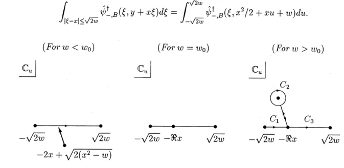
Lemma 3 suggests that some difficulty may arise when $w\geq w_{0}=\mathrm{d}\mathrm{e}\mathrm{f}(\Re x)2/2+(\propto SX)^{2}$.
Figure 3 actually indicates what phenomenon occurs when $w\geq w_{0}$ with the integral
$\int_{|\xi x|\leq\sqrt{2w}}-(\hat{\psi}^{\mathrm{t}}-,B\xi, y+x\xi)d\xi=\int_{-\sqrt{2w}}^{\sqrt{2w}}\hat{\psi}_{-,B}\uparrow(\xi, X/22X+u+w)du$ .
(For$w<w_{0}$) (For $w=w_{0}$) (For$w>w_{0}$)
$\lrcorner \mathbb{C}_{u}$ $\lrcorner \mathbb{C}_{u}$
$-\overline{\sqrt{2w}\backslash \sqrt{2w}}$ $-\overline{\sqrt{2w}-\Re_{X}\sqrt{2w}}$
$-\sqrt 2w-\Re X$ $\sqrt 2w-$
$-2x+\sqrt{2(x^{2}-w)}$
The corresponding branch point of crosses
the path of integration from below in the complex $u$-plane. (Here we have chosen the
branch of$\sqrt{2(x^{2}-w)}$sothat it maybecome$2x-\Re x$ at $w=w_{0}.$) Hencethe integral in
question, which is a constant multipleof$\psi_{+,B}^{\ddagger}(X, y)$ when $w<w_{0}$ (Proposition 1), is no
longer its analytic continuation for $w>w_{0}$
.
The above integral contributes only to theintegral along the portions $C_{1}(\mathrm{f}\mathrm{r}\mathrm{o}\mathrm{m}-\sqrt{2w}\mathrm{t}\mathrm{o}-\Re_{X})$ and $C_{3}$ ($\mathrm{f}\mathrm{r}\mathrm{o}\mathrm{m}-\Re_{x}$ to $\sqrt{2w}$). To
obtain the Borel sum ofthe WKB solution $\psi_{+}^{\ddagger}$ of (1) we need the analytic continuation
of $\psi_{+,B}^{\iota}(X, y)$. That is, it is necessary to take account ofthe integral along the portion
$C_{2}$ also (cf. Figure 3).
Let us now try to compute more convenient form of the integral along $C_{2}$. In view
of Lemma 1 the integral has the followingform:
(23)
$I_{2}= \frac{1}{\Gamma(\frac{1}{2}+\frac{\lambda}{4})}\int_{C_{2}}\xi^{-}2/3[(s-1)^{-}\frac{1}{2}+\frac{\lambda}{4}F(\frac{1}{4}+\frac{\lambda}{4}, \frac{3}{4}+\frac{\lambda}{4}, \frac{1}{2}+\frac{\lambda}{4};1-s)]|_{s=\frac{y+}{\xi}}x\underline{\xi}du2+\frac{1}{2}$.
Note that the variable $s$ becomes $0$ at the branch point $u_{*}$
.
This means that theintegrand of $I_{2}$ has a singularity at $u_{*}$
.
The
behavior of the integrand there can befigured out by the following classical formula for hypergeometric functions:
$F(\alpha, \beta,\gamma;1-S)$ $=$ $\frac{\Gamma(\gamma)\mathrm{r}(\alpha+\beta-\gamma)}{\Gamma(\alpha)\Gamma(\beta)}s^{\gamma-\alpha-}F\beta(\gamma-\alpha,\gamma-\beta,\gamma-\alpha-\beta+1;s)$
$+ \frac{\Gamma(\gamma)\Gamma(\gamma-\alpha-\beta)}{\Gamma(\gamma-\alpha)\mathrm{r}(\gamma-\beta)}F(\alpha, \beta, \alpha+\beta-\gamma+1;s)$
(cf. [BMP,
\S 2.10]).
Sincethe secondtermof the right-handsideis holomorphic at$s=0$,only the first term contributes to the integral $I_{2}$. Making use of this formula together
with Kummer’s relation
$(1-S)^{\gamma\beta}-\alpha-F(\gamma-\alpha, \gamma-\beta, \gamma;s)=F(\alpha, \beta, \gamma;S)$
($[\mathrm{B}\mathrm{M}\mathrm{P}$, Formula (23) in
\S 2.1]),
and paying some attention to the determination of thebranch of $(s-1)^{-}1/2+\lambda/4$ and of $s^{-1/2-\lambda/4}$, wefind
$I_{2}$ $=$ $e^{-i\pi(-\frac{1}{2}+} \frac{\lambda}{4})(^{2i}e-\frac{1}{2}-\frac{\lambda}{4})-\pi(1)\frac{\Gamma(\frac{1}{2}+\frac{\lambda}{4})}{\Gamma(\frac{1}{4}+\frac{\lambda}{4})\mathrm{r}(\frac{3}{4}+\frac{\lambda}{4})}$
It follows from the well-knownformula $\Gamma(1/2+z)\Gamma(1/2-z)=\pi/\cos\pi z$ and (22) that
$e^{-i\pi \mathrm{t}\frac{1}{2}}-+ \frac{\lambda}{4})(^{2}e-\frac{1}{2}-\frac{\lambda}{4})-i\pi \mathrm{t}1)\frac{\Gamma(\frac{1}{2}+\frac{\lambda}{4})}{\Gamma(\frac{1}{4}\dagger\frac{\lambda}{4})\Gamma(\frac{3}{4}+\frac{\lambda}{4})}=\frac{-i\sqrt{2\pi}2\lambda/2}{\Gamma(\frac{1}{2}-\frac{\lambda}{4})\Gamma(\frac{1}{2}+\frac{\lambda}{2})}e^{-i\lambda/2}\pi$.
Hence we finally obtain
(24) $I_{2}$ $=$ $\frac{-i\sqrt{2\pi}2^{\lambda/2}}{\mathrm{r}(\frac{1}{2}-\frac{\lambda}{4})\mathrm{r}(\frac{1}{2}+\frac{\lambda}{2})}e^{-i\pi\lambda/2}$
$\cross\int_{\xi_{0}}^{\xi_{\mathrm{r}}}\xi^{-}2/3[s^{-\frac{1}{2}-\frac{\lambda}{4}}F(\frac{1}{4}-\frac{\lambda}{4}, \frac{3}{4}-\frac{\lambda}{4}, \frac{1}{2}-\frac{\lambda}{4};s)]|_{s=\frac{y+x\xi}{\xi^{2}}+\frac{1}{2}}d\xi$
where $\xi_{*}=-X+\sqrt{2(x^{2}-w)}$
.
It is then natural to ask “What is this integral?” The answer is the following: The
steepest descent path $\Gamma$ of $\Re\varphi$-intersects a Stokes curve of (9) at a point $\xi_{0}$
.
We nowdraw the steepest descent path, denoted by $\tilde{\Gamma}$
, of $\Re\varphi_{+}$ from this crossing point $\xi_{0}$ (cf.
Figure 1, where $\tilde{\Gamma}$
is written by dotted lines) and consider the inverse Fourier-Laplace
transform of the Borel resummed WKB solution $\hat{\Psi}_{+}^{\uparrow}$ integrated along
$\tilde{\Gamma}$
:
(25) $\int_{\tilde{\Gamma}}\exp(\eta x\xi)\hat{\Psi}_{+}\dagger(\xi, \eta)d\xi=\int_{\tilde{\Gamma}}\exp(\eta x\xi)(\int_{-\xi^{2}/2}^{\infty}\exp(-\eta Z)\hat{\psi}^{\dagger}+,B(\xi, z)dZ)d\xi$.
Similarly to the case of $\hat{\Psi}^{\uparrow}$
let us introduce new variables ofintegration by
(26) $x \xi+\frac{1}{2}\xi^{2}=x\xi_{0}+\frac{1}{2}\xi_{0}^{2}-\tilde{u}(\tilde{u}\geq 0)$, $z=- \frac{1}{2}\xi^{2}+\tilde{v}(\tilde{v}\geq 0)$
and employ the same change of variables (13). Noting that
(27) $y=z-x \xi=\tilde{v}+\tilde{u}-(x\xi_{0}+\frac{1}{2}\xi_{0}^{2})=-\frac{1}{2}x^{2}+w_{0}+\tilde{u}+\tilde{v}$,
we then obtain the following expression of (25):
(28) $\int_{y=}\frac{1}{2}2\mathrm{x}\mathrm{e}\mathrm{p}w=w0^{-x+w}+\overline{u}+\overline{v}\geq w0(-\eta y)(\int_{w-}w\mathrm{o}\geq\overline{u}\geq 0y\hat{\psi}_{+,B}\uparrow(\xi,+x\xi)d\xi)dy$
.
The endpoints $w-w_{0}$ and $0$ of the inner integral respectively correspond to $\xi_{*}$ and $\xi_{0}$
in the $\xi$-variable. Hence, in view of Lemma 1 again, the inner integral of (28) can be
rewritten as
(29) $\frac{1}{\Gamma(\frac{1}{2}-\frac{\lambda}{4})}\int_{\xi}^{\xi_{0}}.\xi-2/3[s^{-\frac{1}{2}}-\frac{\lambda}{4}F(\frac{1}{4}-\frac{\lambda}{4}, \frac{3}{4}-\frac{\lambda}{4}, \frac{1}{2}-\frac{\lambda}{4};s)]|_{s=*_{\epsilon^{x}}\frac{1}{2}}s_{+}d\xi$ .
Proposition 2 When $w>w_{0_{J}}$ the following relation holds:
(30) $\sqrt{2\pi}\psi_{+,B}^{\ddagger}(x, y)=\int_{1\xi-}x|\leq\sqrt{2w})\hat{\psi}\uparrow-,B(\xi,$$y+x\xi d\xi+I_{2}$,
where
(31) $I_{2}= \frac{i\sqrt{2\pi}2^{\lambda/2}}{\Gamma(\frac{1}{2}+\frac{\lambda}{2})}e^{-i}\pi\lambda/2\int_{w-w_{0}}\geq\tilde{u}\geq 0)\hat{\psi}_{+,B}\dagger(\xi,$$y+X\xi d\xi$
.
Corollary 1 The inverse Fourier-Laplace
transform of
(a linear combination of) Borelresummed $WI\mathrm{f}B$ solutions
defined
by(32) $\int_{\Gamma}\exp(\eta x\xi)\hat{\Psi}^{\uparrow}(\xi, \eta)d\xi+\frac{i\sqrt{2\pi}2^{\lambda/2}}{\Gamma(\frac{1}{2}+\frac{\lambda}{2})}e-i\pi\lambda/2\int_{\tilde{\Gamma}}\exp(\eta_{X}\xi)\hat{\Psi}_{+}\uparrow(\xi,\eta)d\xi$
coincides with $\sqrt{2\pi}\Psi_{+}^{\ddagger}(x, \eta)$, the Borel sum
of
a $WI\mathrm{f}B$ solution $\sqrt{2\pi}\psi_{+}^{\ddagger}$of
the originalequation (1).
Remark 2. The constant $i\sqrt{2\pi}2^{\lambda/2}e^{-i}\pi\lambda/2/\Gamma(1/2+\lambda/2)$ before the second term of
(32) is exactly equal to that appearing in the connection formula for $\hat{\Psi}^{\underline{\dagger}}$
on thepositive
imaginary axis (cf. [Tl, Proposition 5]).
Summing up, we can state the conclusion of this note as follows:
CONCLUSION: To discuss the Fourier-Laplace transform of Borel resummed WKB solutions of the harmonic oscillator, the usual steepest descent method
is insufficient. However, if we take into account a “bifurcated” steepest
descent path (like$\tilde{\Gamma}$
) besides usualsteepest descent paths, then the (inverse)
Fourier-LaplacetransformofBorel resummed WKB solutions actually gives
us the Borel sum of a suitable WKB solution.
Thissuggests that the conclusion shouldhold for general ordinary differentialequations
with arbitrary polynomial coefficients. Generalization of this result to more general
equations shall be discussed in our forthcoming papers.
References
[AKTI] T. Aoki, T. Kawai and Y. Takei: New turning points in the exact WKB
analysis for higher-order ordinary differential equations, Analyse alg\’ebrique
[AKT2] –: On the exact WKB analysis for the third order ordinary differential equations with a large parameter, Asian J. Math., 2(1998), 625-640.
[BMP] A. Erd\’elyi et al.: Higher Transcendental Functions. Bateman Manuscript
Project, Vol. I, California Institute of Technology, $\mathrm{M}\mathrm{c}\mathrm{G}\mathrm{r}\mathrm{a}\mathrm{W}$-Hill, 1953.
[BNR] H. L. Berk, W. M. Nevins and K. V. Roberts: New Stokes linesin WKB theory,
J. Math. Phys., 23(1982), 988-1002.
[BH] M. V. Berry and C. J. Howls: Hyperasymptotics for integrals with saddles,
Proc. Roy. Soc. London, A 434(1991), 657-675.
[H] C. J. Howls: Hyperasymptotics for multidimensional integrals, exact
remain-der terms and the global connection problem, Proc. Roy. Soc. London, A
453(1997), 2271-2294.
[T1] Y. Takei: An explicit description of the connection formula for thefirst Painlev\’e
equation, Toward the Exact WKB Analysis of Differential Equations, Linear
or Non-Linear, Kyoto Univ. Press, 2000, pp. 271-296.
[T2] –: Integral representation for ordinary differential equations of Laplace
type and exact WKB analysis, in preparation.
[U1] K. Uchiyama: On examples of Voros analysis of complex WKB theory, Analyse
alg\’ebrique des perturbations singuli\‘eres. I, Hermann, 1994, pp. 104-109.
[U2] –: Graphical illustration of Stokes phenomenon of integrals with saddles,
Toward the Exact WKB Analysis of Differential Equations, Linear or