ANALYSIS OF A DYNAMIC ASSIGNMENT QUEUEING MODEL WITH POISSON CLUSTER ARRIVAL PROCESSES

Vol. 41, No. 2, June 1998

ANALYSIS OF A DYNAMIC ASSIGNMENT QUEUEING MODEL WITH POISSON CLUSTER ARRIVAL PROCESSES

Toshihisa Ozawa Takuya Asaka N T T Multimedia Networks Laboratories

(Received August 22, 1996; Final December 10, 1997)

Abstract We consider a dynamic assignment queueing model with multiple packet classes, which has a number of queues, each with its own server. This model arises from the output buffer control of an ATM-based packet switching system, which is connected to another system via multiple links. Each packet is divided into cells and transmitted by cell-by-cell transmission through the links. Such packet arrival processes can be modeled as Poisson cluster arrival processes. An arriving packet is assigned to one of the queues according to a dynamic packet assignment scheme, which is a variation of the shortest queue policy and tries to assign buffer space and/or transmission bandwidth fairly to each class when the system is congested. We derive an approximation of the packet loss probability by using a decomposition method and an asymptotic of the cell loss probability. Its accuracy is examined in comparison with simulation results. The results of this paper can be used for dimensioning the buffer sizes of the ATM-based packet switching sys tems.

1. Introduction

Recent developments in computer communication require higher speed interconnection ser- vices between local area networks (LANs) over wide geographical areas. One way t o pro- vide these services is t o build a packet overlay network on top of an asynchronous transfer mode (ATM) backbone network by using ATM-based packet switching systems, whose typ- ical examples are connectionless servers (CLSs) [3, 4, 13, 171. In such a packet overlay network, ATM-based packet switching systems are interconnected via permanent virtual circuits (PVCs). Each packet is divided into cells of 53 bytes in d a t a length including the headers and is transmitted by cell-by-cell transmission through the PVCs. If ATM adap- tation layer (AAL) type 3 or type 4 is used in the network, the first and last cells of each

packet can be detected by using the values of the segment types (STs) of cells, and if AAL type 5 is used, those cells can be detected by using the values of the payload types (PTs) of cells. Hence the ATM-based packet switching systems can identify individual packet S without reassembling the packets. Furthermore, by reading packet destination addresses directly from the first cells of the packets, they can also route and forward the packets by high-speed cell-by-cell processing without reassembling the packet S.

When we attempt to build such a packet overlay network, we must sometimes use multi- ple PVCs t o connect ATM-based packet switching systems because of technological and/or economical restrictions [5, 71 (Fig. 1). In this case, a packet assignment scheme for multiple PVCs is necessary to construct a n output buffer control mechanism used in the ATM-based packet switching system. Here, assigning a packet to a queue corresponds to assigning all the cells of the packet to the same queue1. Such an output buffer control mechanism together 'Cell assignment schemes of this type make it possible for ATM-based packet switching systems to

A Dynamic Assignment Queueing Model

PSS: ATM-based Packet Switching System

Figure 1: A packet overlay network.

Queues with servers

Input cells

. . .

Figure 2: A parallel server model.

with multiple PVCs can be modeled as a parallel server model, where servers correspond t o the PVCs and each server has its own cell buffer (Fig. 2). One of the typical packet assignment schemes is the shortest queue policy [19], which is a dynamic packet assignment scheme and randomly assigns a n arriving packet t o one of the shortest queues. Note t h a t in this paper the queue length is counted including the cell being served a t the server. This policy intends t o use the servers more efficiently and t o make the packet loss probability smaller.

However, when the shortest queue policy is used and one user sends many packets a t a

time, packet delays for other users may become longer and their many packets may be lost. Hence we consider the case of multiple packet classes, each corresponding t o a user, and a variation of the shortest queue policy in order t o assign buffer space and/or transmission bandwidth fairly to each class when the system is congested. Here each class can be identified by, for example, the source addresses (SAS) of the packets, their destination addresses (DAs), and the SA-DA pairs, and it can also be identified by the virtual channel identifiers (VCIs), the virtual pat h identifiers (VPIs)

,

and/or the multiplexing identifiers (MIDs) of the cells of the packets [ l , 21. In our packet assignment scheme, a t the arrival of a packet if there exist no idle servers and there exist packets of the same class in t h e system, the arriving packet is assigned t o the queue t o which the latest packet of the same class was assigned. T h e scheme is composed of the following cell-based packet assignment rules.

(i) At the arrival of the first cell of a packet if there exist no cells of the same class in the system, the cell is randomly assigned t o one of the shortest queues.

(ii) At the arrival of the first cell of a packet if there exist cells of the same class in the identify each packet, whose cells are transmitted through a common PVC, by using the values of the STs or the P T s of cells. Cell assignment schemes that can assign the cells of each packet to different queues are the other type, and they require ATM-based packet switching systems to identify the individual packets whose cells may be transmitted through different PVCs [7]; This makes it difficult to construct dynamic assignment schemes of the latter type. Hence we consider only those of the former type in this paper.

system and if there are no idle servers, then the cell is assigned t o the queue to which the latest packet of the same class was assigned.

(iii) At the arrival of the first cell of a packet if there exist cells of the same class in the system and if there exist idle servers, then the cell is randomly assigned to one of the queues of the idle servers.

(iv) A cell which is not the first cell of a packet is assigned to the same queue as the first cell of the packet.

Rule (i) corresponds t o the shortest queue policy. Rule (ii) makes packets of each class apt to be assigned t o just one queue when the system becomes congested, and these rules lead to fairness among classes. Rule (iii) contributes t o using servers more efficiently. Rule (iv) makes this cell assignment scheme a packet assignment scheme.

The input process of each class can be modeled as a Poisson cluster arrival process [14]. Packets, which are called clusters in the Poisson cluster arrival process, arrive a t the system via a Poisson process, and each packet is decomposed into a certain number of cells, which are called customers in that arrival process. These cells of the packet are usually assumed t o arrive a t the system with constant intervals2 and are sent out through a

. We approximately analyze this parallel server model with finite buffers and derive an approximation for the packet loss probability. Here a packet is assumed t o be lost when a t least one cell of the packet is lost in the network, since t h a t packet cannot be assembled a t the destination.

The rest of the paper is constructed as follows. In Section 2 we describe our parallel server model in detail. In Section 3 we introduce an approximate model for a single queue of the original model. In Section 4 we analyze the approximate model and obtain a n approximation for the packet loss probability. In Section 5 the accuracy of the approximation is discussed through numerical experiments, and an improvement of the approximation of the packet loss probability is proposed.

2. Model description

Here we present a rigorous definition of our parallel server model with multiple packet classes. Our model is described as follows (see Fig. 2).

There are S queues. Each queue behaves like a - / D / l / K model, where service times are equal t o a constant A

(>

O), which corresponds t o the time taken t o transmit one cell, and

K is the buffer size including the service position. In each queue cells are served according t o the first-in-first-out (FIFO) discipline.

Let N be the number of packet classes. We only consider a symmetric case, where the arrival processes of individual classes are mutually independent and subject to a common stochastic law. Packets in each class arrive a t the system via a homogeneous Poisson process with intensity Ao. The sizes (the number of cells) of packets in all classes are i.i.d. random variables and we denote by X. a generic random variable representing the packet size. Let the time between consecutive cell arrivals in the same packet be equal t o a constant

8

(>

0). Here 1/6 corresponds to the cell transmission speed of PVCs connecting user routers t o ATM-based packet switching systems, while l / A corresponds t o that of PVCs interconnecting the ATM-based packet switching systems. The former speed is usually less than or equal t o the latter one; However we sometimes use PVCs of the same speed t o build a packet overlay networks. Hence we assume that they have the same value (i.e. A =

6).

We will refer t o an arrival process of this type as a Poisson cluster arrival process [l41 and

A Dynamic Assignment Queueing Model 199 denote by A 4 ^ y D ) , where

B ( X ,

D) represents the characteristic of each packet as in [ll];

X means that the distribution of the packet (cluster) size is general and D means that the cell (customer) arrival intervals in the packet are determinate. Packets (and hence cells) are assigned t o one of the queues according t o the shortest-queue-type packet assignment scheme described in the previous section. A cell is lost if it arrives a t the system when the buffer of the assigned queue is full. A packet is considered t o be lost if a t least one cell of the packet is lost.

For convenience of description, in the following sections, A and 8 are set equal to the unit time length (i.e. A = 8 = 1).

3. Decomposition of the model

The original model introduced in the preceding section is very complicated, and it seems difficult to get exact results for performance measures. In order to derive an approximation for the packet loss probability in the next section, here we shall decompose the original model into S independent

M^'^/D/~/K

models each of which approximately describes the stochastic behavior of the corresponding queue. Hereafter we assume that all processes considered in this section are in steady states.

For j = 1 , 2 ,

...,

S, let Aj(t) be the number of packets that are assigned to queue j during the interval (0, t], Gj(t) be the stochastic intensity of &(t) a t time t , and Lj(t) be the queue length of queue j , or equivalently the number of cells being served or waiting in queue j, a t time t . First, we derive the conditional expectation of Gj (t) given that L j (t)

>

0; E[i$(t)

1

LAt)

>

01 is decomposed as follows:

The conditions "Lj(t)

>

0" and

"nLl

!(Lt(<)

>

0) = 0" mean that, a t time t , there exist empty queues but queue j is not empty. According t o Rules (i) and (iii), the expectation in the first term on the right side of equation (3.1) is, therefore, zero. The expectation in the second term is given as

because the summation of the left side of equation (3.2) on j is equal to NAo and S queues are symmetric. Substituting (3.2) into (3.1), the conditional expectation of G j (t) is given as

Note that, since Rule (ii) is not used for deriving equation (3.3) explicitly, another expression for the expectation of Gj(t) seems t o be needed to approximate the packet arrival rate under the condition where the system is congested, in other words, where the value of Lj(t) is large. This will be discussed again in Subsection 5.2.

T h e conditional probability on the right side of formula (3.3) is represented as

Since S queues are symmetric, the denominator on the right side of this equation is given by

where bLK) denotes the cell loss probability. The numerator is the probability that all the servers are busy, and its approximation is derived as follows. Consider a modification of the parallel server model, where each packet is regarded as one customer and his service time is equal t o the size of the packet. In this modified model, customers of each class arrive via a Poisson process with intensity Ao, an arriving customer is assigned t o one of the queues according t o the same scheme, and each queue behaves like a - / G / l / K . Here we consider a case where the capacities of the buffers are infinite. Since, in the original model, cell arrival intervals in each packet are equal to the constant service time, the probability that all the servers are busy in the original model is equal t o that probability in the modified model. Hence we approximate that probability of the original model by using the probability that all the servers are busy in an M/G/S/oo model, where the arrival rate is equal t o ( l - bLK) NAo and the service time distribution is the same as that of Xo. From [g], this probability of the M/G/S/oo model can be approximated by using the corresponding probability of a n M/M/S/oo model, where the arrival rate is the same as that of the M/G/S/oo model and the mean service time is equal to EIXo]. As a result, we obtain the following approximation:

where

From formulas (3.4), (3.5), and (3.6), the following approximation is obtained.

S -5-1

l ( L t ( t )

>

0) = 1 Sao p0

(S - l ) ! (S -

no)

'

A decomposed M ~ ( ~ ^ / D / ~ / K model is given as follows: let A be the packet arrival intensity in the model. From formulas (3.3) and (3.9), A is given by

~ A ~ i i i - ~ &

A

=

(S

- l ) ! (S - Go) '

T h e distribution of packet sizes and the value of service times of cells in the decomposed model are the same as those in the original model.

A Dynamic Assignment Queueing Model 201

E

[%

(t)

1

L j (t)

>

01 is the conditional mean arrival intensity of packets given that L j (t)

>

0; however, we use the same value for the case when L j ( t ) = 0. T h e reason is as follows. From Remark 1 below, both the cell loss probability and the packet loss probability are independent of the packet arrival intensity during idle periods because the packet arrival processes are assumed t o be Poissonian and the beginning point of each busy period is a

regeneration point for the cell arrival processes.

[Remark l] Consider a G / G I / c / K model. Let ~ ( t ) be the number of customers that arrive a t the system during an interval (0, t] and be the service time of the n t h arriving customer. Suppose that the beginning point of each busy period is a regeneration point for ~ ( t ) . Let B{t) be the number of customers that overflow from the system during an interval (0, t]. Since B{t) can be generated from { ~ ( s ) , S

5

t} and

{L

n

<

~ ( t ) } , the beginning point of each busy period is also a regeneration point for ~ ( t ) . Therefore, from the property of renewal-reward processes

[a],

the overflow probability

b

is given by

where is the number of customers that arrive during a busy cycle (a busy period and the subsequent idle period), and

B.

is the number of customers that overflow during the busy cycle. Because all the arrivals and overflows in each busy cycle occur in the busy period, both

A0

and go are independent of the probability law of A f t ) during the idle period of the busy cycle. Therefore,

b

is also independent of the probability law of ~ ( t ) during idle

periods. D

4 An approximate analysis of a discrete-time version of the M * ( ~ ? ~ ) / D / ~ / K model

In this section, we consider a discrete time version of the M ~ ( ~ ~ ~ ) / D / ~ / K model; cells arrive and depart only a t discrete time points {O, 1, 2, ...

}.

We further assume that departures occur before arrivals a t the same time point. For the case where the distribution of X. is geometric, the cell loss probability was derived in [ l l ] . Here we assume that X. is bounded above and do not assume that its distribution is geometric. An approximation of the packet loss probability is derived in the following three steps: (1) An upper bound of the cell loss probability is obtained. (2) Using this upper bound, a n approximation of the cell loss probability is derived. (3) The packet loss probability is approximated using the cell loss

probability.

4.1. Upper bound of the cell loss probability

Let a p ( n ) be the number of packets arriving a t time n. Then {ap(n)} are i.i.d. random variables subject to a Poisson distribution with mean A. Let X j be the size (the number of cells) of the j t h arriving packet and assume that each Xj has the same upper bound gmaz. Packets are numbered sequentially, with the first packet t h a t arrives after time zero having the number zero. Let p be the traffic intensity defined as p A EIXo]. Let a c ( n ) be the number of cells that arrive a t time n. When the j t h packet arrives a t time n , its cells arrive sequentially a t n , ( n

+

l ) , ..

.,

( n

+

X, - 1). Let I p ( n ) be the number of active packets that

have cells arriving after time n and Rc{$ n ) be the number of residual cells of the i t h active packet for i = 1, 2,

...,

I p ( n ) ; for example, if a packet of size Xk arrives at time n when the system is empty, then R c ( 1 , n ) = Xk - 1, R c ( l , n

+

1) = Xk - 2, and so on. Let Z ( n ) be a

vector indicating the number of active packets and the number of residual cells:

Since { Z ( n ) } forms a Markov chain and ac{n) satisfies equation

{ a c ( n ) } can be considered as a discrete-time Markov Aadditive process (MAP) with the underlying Markov chain { Z ( n )

}

.

We first analyze a n ~ ~ ( ~ ~ ~ ) / D / l / o c l model, which has the same arrival process and service times as the M * ( ~ ~ ~ ) / D / ~ / K model, but the buffer capacity is infinite. For each n

>

0, consider a queueing process that began a t time -n, and let L o ( n ) be the number of cells in the system at time zero. We introduce the following notations:

Mo{n) E: L o ( n ) - ac ( 0 ) for n

>

0,

u ( n ) a c ( - n ) - 1 for n

>

0 , n

U ( n )

=

x u ( j ) f o r n 2 1 , U(O)=O.

]=l

From the definition of the process { u ( n ) } , this process becomes a discrete-time MAP with the underlying Markov chain { Z ( n ) } . Renumbering the states of { Z ( n ) } such that the state space becomes

P,

the kernel of the MAP and its transform are defined by

where

Loin} and M o ( n ) are represented by U (-) in the following manner:

+ + +

L0 ( n ) = [ ~ ( l )

+

[ u ( 2 )

+

+

[+)l

] ]

+

ac(O)

= max U ( j )

+

ac (0)) (4.11)

057 5n

M o ( n ) = o<j<n max U ( j ) . (4.12)

Under some suitable conditions foi and MQ, are obtained as follows:

{ac ( n ) ) , the stationary versions of L. ( n ) and M o ( n ) , L.

lim MO(%) = sup U ( n )

,

n+m _{n â ‚ ¬}

lim L o i n ) = MO

+

ac ( 0 ) . n+m

A Dynamic Assignment Queueing Model 203

We further introduce the following notations:

A(n; S)

=

log ~ [ e ' ~ ( ~ ) ] for n

>

0 and 0 C ¥R. (4.15) A(0)

=

lirn n - l ~ ( n ; 0) for n

>

0 and 0

R,

n-im (4.16)

0' sup{@

1

A($)

<

O}. (4.17)

Then, using the results of [6], an upper bound of the tail distribution of MO is given by the following theorem.

[Theorem l] [6] If E [ u ( l ) ] = p - 1

<

0, then

Pr(Mo

>

k)

5

4 0 ) e-'* for k

>

0 and S E [O, 61'1, (4.18) where p(0) is the essential supremum

p(0)

=

sup ( X : P r

(

l(+)

>

0)

>

>

()

f2i.i (6)

1.

and ( ~ 4 0 ) ) is the right eigenvector of the matrix

(pn-

(0)) corresponding t o the simple max- imal eigenvalue eA('). The vector (vi(@)) is positive and bounded above.

Since [Lo - l]+ = [Mo

+

u(O)]+

A

MO, an upper bound of the tail distribution of L. is

given as

Pr(Lo

>

k) = Pr([Lo - l]+

>

k - 1) = Pr(Mo

>

k - 1)

<

- p(@ e-'('-l) f o r k

>

1 and 0 _E [O,

0*}.

(4.20)

Let

br'

be the cell loss probability in the M ^ ' ( ~ ~ ~ ) / D / ~ / K model. Then we have the following theorem.

[Theorem 21

(Proof) See Appendix.

Theorem 2 and (4.20) directly lead to an upper bound of b K ) as

b?)

5

y(<l)e-*"" for 0 C [O, S*]. (4.22)

4.2. Approximation of the cell loss probability

On the right side of inequality (4.22), O* is easily calculated according t o Proposition 1

below; however, it is difficult to calculate p(@) because the eigenvector (vi(@)) should be calculated. Hence we try to approximate the cell loss probability. From [6], the asymptotic decay rate of the distribution of MO is

-Q*,

i.e. limK- K 1 log Pr(Mo

2

K) = -Q*. From this and Theorem 2, it is proved that the asymptotic decay rate of bLK) with respect to K

is bounded by -g*, as follows:

lim K-' log b,$?)

5

lim K-' log(p-l Pr(Lo

2

K

+

1))

K- K->m

= _lim

_K-'{-

_{log p}

+

_{log Pr(Mo K)} = -0'.}

From this result we propose the following approximation:

bg' is the cell loss probability of the

MB^X'D^/D/~/~

model, and it can be obtained by using the fluid flow approximation as follows. Consider a n M/G/oo model, where the arrival rate is equal t o A and the service time distribution is the same as that of Xo. Let Loo(t) be the number of cells in the system at time t . We assume that, in this M / G / m model, work is lost a t a rate (Loo(t) - 1) when Loo(t)

>

1, and let the volume of lost work correspond to

the number of lost cells in the MB<Â¥X^/~/l/ model. As a result, b g ) is approximately

lim f ' [ L a ( s ) - 11+ ds t+oo

S;

L^{s) ds given by the following formula:

b p Ã

The value of 0* can be calculated according t o the following proposition.

[Proposition l] Assuming p = A EIXo]

<

1, the value of 6* is obtained as the unique positive root of the equation

where [ ( z )

= E[

zxO 1. The root can be easily calculated using usual numerical methods, such as Newton's method or the binary search method.

(Proof) Let us consider a discrete-time version of an M x / ~ / l / m model, where all the cells of each packet arrive a t the same time, not with regular intervals. T h e packet arrival process, packet sizes, and service times are the same as the discrete-time version of the

M^M/D/I/K

model. For this ~ - " / D / l / o o model, let a:(n) be the number of cells that arrive a t time n , and let uO(n), U O ( n ) , AO(n; (?), and AO((?) be defined in the same manner as u(n), U ( n ) , A(n; (?), and A((?) in the previous subsection, respectively. This time {a:(^-)} are i.i.d. random variables subject to a compound Poisson distribution.

Since the packet sizes are bounded above by gmax, we have

Hence the following inequality holds:

log ~ [ e ^ ' ( ~ )

]

+

log E[ e-6u0(gmax)

]

_<

- log E[ eeU-)

]

5

log E

[

e6u0(n)

1

+

log E[ e6u0(gmax)

]

. (4.27) Dividing each term by n and letting n tend to infinity, the relation A((?) = AO((?) is obtained. Therefore A((?) is given by

A Dynamic Assignment Queueing Model 205

4.3. Approximation of the packet loss probability

Consider the M ~ ( ~ ~ / D / ~ / K model and assume that it is ergodic. Let

A p ( n )

and A c ( n ) , respectively, be the number of packets t h a t arriving during interval [O, n ) and t h a t of cells arriving during the same interval; and let B 3 n ) and B n n ) , respectively, be the number of packets lost during interval (0, n) and that of cells lost during the same interval. A packet is assumed t o be lost when a t least one cell of the packet is lost. Let b$?) and

&LK)

be the packet loss probability and the cell loss probability, respectively. In order t o represent bpK)

( K )

in terms of bc

,

we introduce the mean number of lost cells in a lost packet, K . This is

( K ) ( K )

given by K limn+OO By ( n ) / B p ( n ) . Using K , b { f } is given by

Bp^ (n) where the upper and lower bounds of K are given by

T h e value of K depends on how the cells of a packet are consecutively lost. In [10], it was shown that the lengths of the periods of loss are independent of the buffer size. From this and numerical experiments in the next section, we conjecture that the value of K is almost invariant with respect t o the buffer size K if the value of K is sufficiently large. However, it is difficult t o calculate K except for the case when K = 1. Therefore, we use the value of

K in that case

( K

= 1) a s a n approximation of K. Letting this value of K be K, the following approximation of bLK is obtained from (4.23) and (4.29).

K is approximately obtained a s follows. Consider the M ~ ( ~ " D ^ / D / \ / ~ model, and let a be the probability that a tagged packet is not lost. Using a, K is given by

where b g ) is given by formula (4.24). We approximate the value of a by using the probability t h a t a tagged packet arrives when the system is empty and no other packets arrive a t the system until all the cells of the tagged packet arrive. Since a tagged packet arriving when the system is not empty may not be lost, this approximation underestimates the value of a. Therefore, K is also underestimated by its approximation. Let Yo be the random variable representing a time interval between consecutive packet arrivals. T h e distribution of Yo is exponential with mean A l . The approximation of a is given by

a a ( l - p ( l - b g ) ) ) P r ( X 0 - 1

5

Yo)

00

-

- 1 - p

+

p b y ) e-*-l) p r ( x o = j )

5 . Numerical experiments and an improvement of the approximation

This section explains the accuracy of the approximations for the cell loss probability, the packet loss probability, and the mean number of lost cells in a lost packet K by comparing them with simulation results; it also presents an improvement of the approximation of the cell loss probability for a parallel server model with the shortest-queue-type packet assignment scheme. Hereafter we use two types of packet size distributions in common: one is a unit distribution, whose mean is equal t o 35, i.e. EIXo] = 35; the other is a uniform distribution, whose minimum and maximum values are equal t o 1 and 35, and whose mean is equal t o 18, i.e. EIXo] = 18. The reason why we use the packet size of 35 a s the maximum packet size is that the maximum packet length in the Ethernet is 1518 bytes and a packet of this size is divided into 35 cells when AAL type 3 or 4 is used.

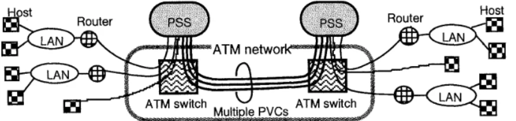
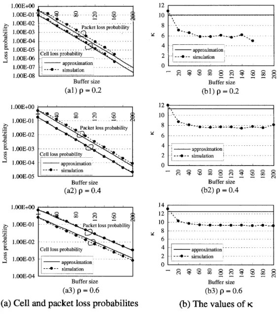
5.1. An

M^'^/D/~/K

model

Figures 3 and 4 show comparisons between approximation results and simulation results for the cell and packet loss probabilities and K in an M ~ ^ X ~ ~ ) / D / ~ / K model. In each case, packet arrival intensity A is determined t o make the traffic intensity p

(=

A EIXo]) be equal to a given value.

Cell loss probability

From Figs. 3(a) and 4(a), we see t h a t the approximation of the cell loss probability is sufficiently accurate for all cases.

The mean number of lost cells in a lost packet: K

From Figs. 3(b) and 4(b), we see that, for all cases, K is underestimated by its approx- imation when the value of the buffer size K is near one, and it is overestimated by its approximation when the value of K is large; the reason for the former was explained in Subsection 4.3. From these experiments, we propose the following conjecture about K: the value of K is rapidly decreasing as K is increasing, and it converges t o some value. If we obtain the value t h a t K converges to, it is expected t o improve the approximation.

Packet loss probability

From Figs. 3(a) and 4(a), we see that the approximation of the cell loss probability is also sufficiently accurate for all cases. Since the approximations of the cell loss probability and K make the approximation of the packet loss probability, the approximation errors of the packet loss probability result from those of the cell loss probability and K . From these experiments, the errors of K do not affect the accuracy of the approximation of the packet loss probability so much.

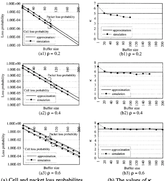
5.2. A parallel server model and an improvement of the approximation

Figure 5 shows comparisons between approximation results and simulation results for the cell and packet loss probabilities in a parallel server model with the shortest-queue-type packet assignment scheme. Since

0.0

in formula (3.10) contains the cell loss probability

&LK,

we here use a n iteration to obtain the approximation results, as follows; Initially, set bc(K) in formula (3.7) t o be zero and calculate an approximate value of the cell loss probability of the parallel server model by using formula (3.10) and the results of section 4; Next, set be ( K ) in formula (3.7) to be this approximate value and calculate a new approximate value of the cell loss probability; Continue this procedure until the difference between a new approximate value of the cell loss probability and the previous one becomes sufficiently

A Dynamic Assignment Queueing Model

Buffer size

(al) p = 0.2

Cell loss probability

Buffer size (a2) p = 0.4

Cell loss probability

l- approximation !

l - -

simulation ,

l

Buffer size

(a3) p = 0.6

(a) Cell and packet loss probabilites

-

, ... I- approximation ; .! * simulation l . . - - . - . - - - - I 12 4 1 10 8 Y 6 4 2 0 0 1 J

s

s

s

s

g

~

~

~

g

g

Buffer size (b2) p = 0.4

:.,

..'... . . . *-. - - . . - . - ?:!.e+L*--a .=*=- a c - - - . - - - - . . -* -l p -- ... l- approximation, --! - - a - - simulation ; -~ - - - - - ~- ~ - - -~ ~ ~~ l , , Buffer size - s g g g o o 0 0 0

ocs¥5F^oOo

Buffer size (bl) p = 0.2

(b) The values of

K

Figure 3: An M ~ ( ~ T ~ ) / D / ~ / K model ( X o = 35: constant).

small. From this figure we see that our approximations are accurate only when the buffer size K is near one. T h e reason for this is considered as follows: if the number of cells in queue j is greater than one, a t least two packets have recently been assigned t o the queue and a t the time point when the latest packet was assigned t o the queue all the servers in the system were busy. This means that the next packet of the same class a s the latest packet is probably assigned t o the same queue according t o Rule (ii). In such a situation, it is considered t h a t the conditional expectation of Gj (t), E [Gj ( t )

1

L j (t)

>

01, can be represented a s the following formula more accurately than formula (3.3).

N - S S E [Gj(t)

1

L j ( t )

>

01 A0

+

p S l ( L i ( t )

>

0) = 1 ( N -

s ) G - ~ @ ~

= A n + (S - l ) ! (S - Go)

Buffer size

(al) p = 0.2

0 0 0

.m . H . . .. Q . . . .

ket loss probability - . . .

. . . .

Cell loss probability simulation ; ~ ~

L--~ ---p-

-Buffer size (a2) p = 0.4

Cell loss probability

I- approximation --- _simulation L-- - -- - l .WE-05 Buffer size (a3) p = 0.6

(a) Cell and packet loss probabilites

^ approximation l 1 ..-a-- _- simulation [

I

Buffer size (bl) p = 0.2 Buffer size (b2) p = 0.4 1 1 - - a - - simulation

~

0

1

- s ? s % g s z g g g

Buffer size (b3) p = 0.6 2 - - approximation . - - a - - _simulation L- - -. -1

(b) The values of

K 0

Figure 4: An M ~ ( ~ . ^ / D / ~ / K model ( X o is uniformly distributed between 1 and 3 5 ) .

On the right side of the first line of the equation, the first term represents that a t least one class is assigned to queue j ; This means that if a n arriving packet of another class is assigned t o queue j, a t least one of other classes is assigned t o each queue. Hence the second term on the right side of the first line contains the factor ( N - S ) / S instead of N / S . Using

this formula, we propose a hybrid approximation, in which the packet arrival intensity is given by formula (3.10) when the value of K is small, and it is given by formula (5.1) when

the value of K is large. Let Al be the packet arrival intensity given by formula (3.10) and

A2 be t h a t given by formula (5.1). When A is given by A I , let 0* and bg' be denoted b y 0:

and b'c\; when A is given by A2, let 0* be denoted by 0;. A new approximation of the cell

loss probability is given by

br)

% ( 1 - / b ( l ) e - @ i ( K - l ) +

bG

e - e ; ( K - l )

c.1 C,2 C.1 1 (5.2)

( 1 )

A Dynamic Assignment Queueing Model 209

and KO log(3/^; (3 is a parameter t o determine the value of K a t which the term of e-';(^-') becomes superior t o the term of e-e"(K1).

approximation

~

--*--

_simulation

Buffer size

(a) N=20, S=10, p = 0.5

Figure 5: A parallel server model with Scheme B': the first versions of the approximations for the cell and packet loss probabilities (Xo = 35: constant).

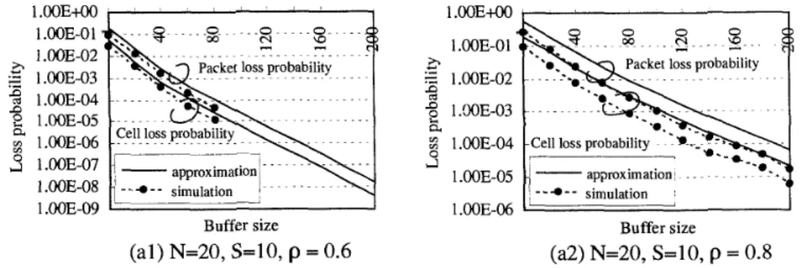
Figures 6 and 7 show comparisons between approximation results and simulation results for the cell and packet loss probabilities in a parallel server model with the shortest-queue- type packet assignment scheme, where the approximation results are calculated by using formula (5.2). The value of (3 is equal t o 10 for all cases. From these figures, we see that the approximations of the cell and packet loss probabilities are rather accurate except for the cases where the packet size distribution is the uniform distribution and the value of p is relatively large.

6. Conclusions

This paper derived an approximation of the packet loss probability for a parallel server model with a dynamic packet assignment scheme, which is a variation of the shortest queue policy. Numerical examples showed the accuracy of the approximations. This approximation is useful for dimensioning the buffer sizes of ATM-based packet switching systems.

Acknowledgments

T h e authors would like t o thank Professor Yukio Takahashi a t the Tokyo Institute of Tech- nology for his insightful advice and discussion. They would also like t o thank the anonymous referees for their valuable comment S.

Appendix A. Proof of Theorem 2

In this appendix, an upper bound of the cell loss probability is obtained using the queueing model with a n infinite buffer. Approximations for cell loss probability have been obtained in other works [12], [15], and [16].

We consider a general discrete-time queueing model denoted by D x / D / c / K : arrivals and departures only occur a t discrete time points {n : n E Z + } , and it is assumed that the departures occur before the arrivals a t the same time point. c denotes the number of servers and K denotes the buffer size including the service positions. Let a., be the number of cells that arrive at time n. The arrival process, a E {an, n E Z+}, is general; that is, an may depend on {aj, j

<

n - l}. Let L? be the number of cells in the system a t time n . T h e queueing process {L^. n E Z+} is given by the following recursive formulas:

simulation l .WE-o7 ---.p-.--- _"1 Buffer size (al) N=10, S=5, p = 0.5 . . . . . . . . . . Buffer size (bl ) N=20, S= 10, p = 0.5 3 % s g ---.-...rÑ. . . approximation ~ ~ simulation ! l.OOE-10 1 "S Buffer size (cl) N=40, S=10, p = 0.5

F--*--

simulation 1 l .(HE-05 Buffer size a 2 ) N=10, S=5, p = 0.7 Buffer size (b2) N=20, S=10, p = 0.7

cket loss probability

. . .

Buffer size

(c2) N=40, S=10, p = 0.7

Figure 6: A parallel server model: cell and packet loss probabilities (Xo = 35: constant). Before proving Theorem 2, the following proposition is presented:

[Proposition A l l ([l81

,

Theorem 9) Consider two queueing models, D X

/

D / C / Ki

and D ~ / D / C / K ^ , which have the same arrival process a. For these models, the following

formula is obtained:

Let

BP

be the number of cells lost a t time n.

BP

where n 6 2+ is given by

T h e cell loss probability b^ is given by S lim BiK)/

Â

£

;

at, and the traffic intensity p is given by p G

$

lirnndm a e / n . Let (p'00)) be the limiting distribution of

the number of cells in the system for the D ~ / D / C / O O model with the same arrival process

A Dynamic Assignment Queueing Model [;l:;y ... probability

^,

--- approximationl - - - ~ ~ - - - ~ - - - - simulation 1 - - - ~ - - - ~ - - - - l .WE-09 1 ' I Buffer size (al) N=20, S=10, p = 0.6 - - . Â ¥ - _simulation ' l .WE-%

I

Buffer size (a2) N=20, S=10, p = 0.8

Figure 7: A parallel server model: cell and packet loss probabilities (Xo is uniformly ( tributed between 1 and 35).

[Theorem 21 (Generalized version) Assuming that the DX/D/c/oo model is sta- ble (i.e. limnAco

-^Â¥'Lw

<

m w.p.1) and

xzoq

= m w.p.1, an upper bound of b^ is obtained as follows:

(Proof) Let

Q,

be defined by

Q,

EE [L;") - K]+ where n E 2+ and Gn by

a,

EE max{O, a, - rnax{O, K - [L^[ - c]'}}

= max{O, min{an, L ; - K}}. (A.6)

To prove that

{Q,}

is the queueing process for a D X / ~ / c / o o model with arrival process

{&I,

Qa

= So and Q n + l =

[Q,

- c]+

+

an+l,

n E

9

are verified as follows:

do = max{O, min{ao, a. - K}} = max{O, a0 - K} = Q0, and

[Q,

- c]+

+

&.+l

= max{O, max{O,

LP

- K } - C}

+

&+l

= max{an+l,

+

£Lco

- K - c}

= max{ [min{a,+l, L^\ - K}]+, [min{a,+l, L^{

-K}]+ + L ^

- K - c}

= max{O, min{a,+l,

L!;\

- K}, L^ - K - c,

m i n { ~ , + ~ ,

~ f f i

- K }

+

L;") - K - c},

where

For the ~ ~ / D / c / o o model with arrival process {Gn}, let dn be the number of cells that departed a t time n. Since dn+i = min{c,

Q,},

Qn = 0 =!> dn+l = 0, and dn+l

5

c, the following inequality is obtained:

Using 1(Qn

>

0) = l([£Lcc - K]+

>

0) = 1(£Lm

>

K), we get

From this formula and Proposition A4.1, we get

n-1 n-1

c -

~ Â £ 1 ~

_>

K )

+

[L^{ - K - c]'

2

_{x m a x { O , min{ae,}

[LE

_{- c ] + + a e - K }}

n-1

>

rnax{O, min{ae,

[LE!

- c]'

+

at - K}

Using this formula and the assumptions, the proof is completed as follows:

S,¡lK+

S?:

l ( ~ ( ~ ) = J')/n ( 1 - K - C]+

<

lim

+

lim [Ln - 1

n+cc - ae/n n-cc

G^

a t

(A. 10)

References

[l] ITU-T Recommendation 1.363: B-ISDN ATM Adaptation Layer (AAL) specification (1994).

[2] ITU-T Recommendation 1.364: Support of the broadband connectionless data bearer service by the B- ISDN (1994).

A Dynamic Assignment Queueing Model 21 3

[3]

G.

J . Armitage and K. M. Adams: Packet reassembly during cell loss. IEEE Network, September (1993) 26-34.

[4] G. Boiocchi, P. Crocetti, L. Fratta,

M.

Gerla, and M. A. Marsiglia: ATM connectionless server: performance evaluation. In H. Perros, G. Pujolle, and Y. Takahashi (eds.): Modelling and Performance Evaluation of ATM Technology (Elsevier Science Publishers

B. V., North-Holland, 1993), 185-195.

[5] C. B. S. Traw and J. M. Smith: Striping within the network subsystem. IEEE Network, July/August (1995) 22-29.

[6] N. G. Duffield: Exponential bounds for queues with Markovian arrivals. Queueing Systems, 1 7 (1994) 413-430.

[7] E. Gustafsson and G. Karlsson: A literature survey on traffic dispersion. IEEE Network, March/April (1997) 28-36.

[8] D. P. Heyman and M. J. Sobel: Stochastic models in operations research Vol. I

(McGraw-Hill Book Company, New York, 1982).

[g] P. Hokstad: Approximations for the M / G / m queue. Oper. Res., 26(3) (1978) 510-523. [l01 S. Q. Li: Study of information loss in packet voice systems. IEEE Trans. on Commun.,

37(11) (1989) 1192-1202.

[l11 M. Miyazawa and G. Yamazaki: Loss probability of a burst arrival finite queue with synchronized service. Prob. in Engineering and Information Sciences, 6 (1992) 201-216. [l21 M. Miyazawa and H. C. Tijms: Comparison of two approximations for the loss proba-

bility in finite-buffer queues. Prob. i n Engineering and Information Sciences, 6 (1993) 19-27.

[l31 T . Ozawa and T . Asaka: Approximation analysis of packet loss probability for a shared output-buffer. Symposium on performance models for information communication net- works, Kyoto (1996) 335-346 (in Japanese).

[l41 K. Sohraby: Delay analysis of a single server queue with Poisson cluster arrival process arising in ATM networks. GLOBCOM '89 (1989) 611-616.

[l51 H. Sakasegawa, M. Miyazawa, and G. Yamazaki: Evaluating the overflow probability using the infinite queue. Management Science, 39(10) (1993) 1238-1245.

[l61 H. C. Tijms: Heuristics for finite-buffer queues. Prob. jn Engineering and Information Sciences, 6 (1992) 277-285.

[l71 S. Ushijima and K. Noritake: A study on virtual LAN service architecture over ATM based connectionless d a t a networks. Technical Report of IEICE, SSE94-135 (1994) 45-50 (in Japanese).

[l81 W. Whitt: Comparing counting processes and queues. Adv. Appl. Prob., 13 (1981) 207-220.

[l91 W. Winston: Optimality of the shortest line discipline. J. Appl. Prob., 14 (1977) 181- 189.

Toshihisa Ozawa

N T T Multimedia Networks Laboratories

3-9-1 1 Midori-cho, Musashino-shi, Tokyo 180-0012, Japan E-mail: [email protected] .co.jp