A Novel Particle Swarm Optimization based Algorithm for Path Optimization in Embedded Systems

全文

(1)Vol.2012-MPS-87 No.1 2012/3/1. IPSJ SIG Technical Report. and/or are highly computational are not suitable for the embedded systems. Therefore, the algorithms which can perform good A Novel Particle Swarm Optimization based Algorithm quality path optimization and require lesser amount of memory and processor speed are desired. for Path Optimization in Embedded Systems The Path Optimization (PO) generally have two or more opti†1 †1 mization objectives and therefore, also called as multi-objective Umair F. Siddiqi, Yoichi Shiraishi †2 shortest path (MOSP) problem1) . The MOSP is an NP hard and Sadiq M. Sait problem1),2) . The objectives in the multi-objective optimization This work presents a fast and memory efficient Particle Swarm Optimizaproblem can be in contradiction to each other and no single sotion (PSO) based algorithm for solving the multi-objective path optimization lution is said to be optimum. Therefore, the multi-objective opproblem. The proposed algorithm uses innovative technique for particles’ distimization algorithms find a set of Pareto optimal solutions. The placement which is based on exploring new sub-paths in the network in-order to improve the particles’ positions. The proposed algorithm is implemented usEvolutionary Computation (EC) algorithms have been predoming C++ and executed on an ARM based embedded system. Its performance inately used to solve the multi-objective optimization problems. is compared with Non-dominated Sorting Algorithm-II (NSGA-II) and Simulated Annealing (SA). The results show that the proposed algorithm has found The population based algorithms work on a population of soluPareto optimal solutions of quality equal to the NSGA-II and better than SA. tions and simultaneously find several solutions. This approach The maximum number of paths which should be stored in the memory during optimization is about half of the NSGA-II. Therefore, it is suitable for impleis suitable for multi-objective optimization problems which have mentation on embedded systems. several Pareto optimal solutions. The Genetic Algorithm (GA) and Particle Swarm Optimization (PSO)6) are examples of population based algorithms. 1. Introduction This work presents a Particle Swarm Optimization (PSO) based algorithm for the PO problem. The proposed algorithm reduces Path Optimization (PO) is a critical operation in many applithe memory requirement to be equal to the size of its Swarm. cations. A large number of applications are executed on small The proposed algorithm has innovative methods for the velocity size embedded systems which have limited amount of memory calculation and displacement of particles. The performance of and computational speed. Navigation systems of intelligent vethe proposed algorithm is compared with Simulated Annealing hicles is an example application which uses less powerful embed(SA)4) and Non-Dominated Sorting Algorithm -II (NSGA-II)3) . ded systems to reduce power consumption. Intelligent vehicles SA works on only one solution and is therefore very memory include electric vehicles, hybrid vehicles and internal combustion efficient. NSGA-II is a popular algorithm for solving the multiengine based vehicles. The algorithms which require high memory objective optimization problems and finding Pareto optimal so†1 Department of Production Science & Technology, Gunma University, lutions. The results show that the proposed algorithm has found Gunma, Japan Pareto optimal solutions of quality better than the SA and equal †2 King Fahd University of Petroleum & Minerals, Dhahran, Saudi Arabia. 1. ⓒ 2012 Information Processing Society of Japan.

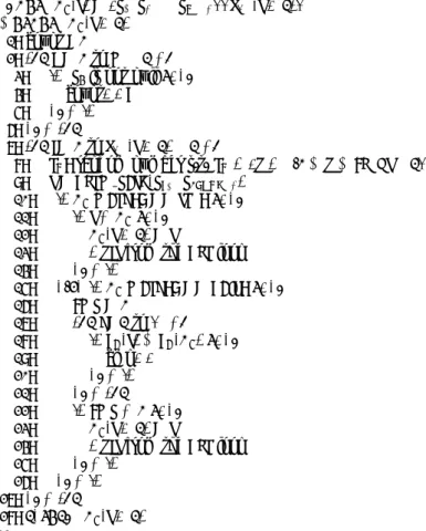
(2) Vol.2012-MPS-87 No.1 2012/3/1. IPSJ SIG Technical Report. to NSGA-II. Its average computation time is at-most 1.42 times of the NSGA-II and 1.47 times of the SA to execute equal number of iterations. . This paper is organized as follows: The second section describes the problem of multi-objective path optimization. Third section presents the proposed algorithm. Fourth section presents the simulation results and discussion. The last section contains the conclusion. 2. Problem Description Let us consider an undirected graph, G = (V, E). The set V contains the vertices or nodes in the graph and set E contains the edges or arcs which join the nodes. Let us consider that the graph contains a total of Nv number of vertices and Ne number of edges. Any edge ei ∈ E is represented as ei = (nx , ny ), where nx is the starting node and ny is the ending node of the edge ei . ei is associated with up-to K weights, i.e., (w1 , w2 , w3 , ..., wK ). A path between a source node i.e., nA and a destination node i.e., nB (nA , nB ∈ V ) is represented as: P = {e0 , e1 , ..., en−1 }, such that: P ⊂ E, e0 = (nA , nx ), en−1 = (ny , nB ), nx , ny ∈ V . Any multi-objective optimization problem can have up-to K objective P functions which are represented as: fk (P ) = ∀ex ∈P ex .wk , for k = 1 to K. The goal of the optimization is represented as: M inimize(f1 (P ), f2 (P ), ..., fK (P )). The solution of any multiobjective optimization problem is a set of Pareto optimal solutions, i.e. SP O = {PS1 , PS2 , ..}, such that any PSi ∈ SP O is a complete path from the source node (nA ) to the destination node (nB ) and is not dominated by any other solution in the set SP O . A solution dominates another solution if it is better than the other solution in at-least one objective function value and the remaining of its objective function values are equal to or better. than the other algorithm. 3. Proposed Algorithm The PSO algorithm was first proposed by Kennedy and Eberhart in 19956) . This section discusses the enhancements in the proposed algorithm in-order to perform memory efficient multiobjective path optimization. 3.1 Representation of Particles In the proposed algorithm, any particle Pj ∈ S, for j= 0 to M − 1 is a complete solution and is represented in an m-dimensional search space (Rm ) as Pj = {p0 , p1 , ..., pm−1 }. The value of any element pi ∈ Pj can be obtained as follows:    nA if i=0 (1) pi = nx if (pi−1 , nx ) ∈ E, nx ∈ V   null if p = {n or null} i−1. B. The first element in any particle Pj contains the source node (nA ), whereas the destination node (nB ) is the last not null element in it. Any two consecutive elements (pi , pi+1 ) represent an edge (ex ∈ E). The objective functions f1 to fK can be applied to individual particles, i.e. Obj(Pj ) = (f1 (Pj ), f2 (Pj ), ..., fK (Pj )). P The function fk (Pj ) = ex ∈Pj (ex .wx ), (where k= 1 to K). 3.2 Initialization The first step in PSO is the initialization of the particles in the Swarm. In this work, the Swarm is initialized to M particles and each particle is a distinct randomly generated path from the source (nA ) to the destination (nB ) node. Fig. 1 shows an algorithm to generate a random path between the two nodes (nA & nB ). 3.3 Find gbest and pbest values In every iteration the values of pbest and gbest solutions. 2. ⓒ 2012 Information Processing Society of Japan.

(3) Vol.2012-MPS-87 No.1 2012/3/1. IPSJ SIG Technical Report. Input: nodes: nA , & nB , G=(V,E), Ne = Number of elements in E Output: Q: A path from nA to nB nodes. 1: W = random(Ne ) 2: Q= Apply Dijkstra’s Algorithm (nA , nB ) 3: return Q Fig. 1. Method to find a random path: f orm path(nA , nB ).. should be updated. The pbest value for any particle Pj consists of K components and is represented as: pbest(Pj (t)) = {lPj 1 , lPj 2 , ..., lPj K }. The values of the components can be determined as: lPj k (t) = arg min(fk (Pj (t))), where t is the itt. eration count, k= 1 to K and j = 0 to M − 1. The global best i.e., gbest has up-to K components and is represented as: gbest = {g1 , g2 , ..., gK }. The value of any component gk ∈ gbest can be computed as: gk = arg min((lPj k )), where j= 0 to M − 1 j. and k= 1 to K. 3.4 Selection of the Pareto Optimal Solutions In every iteration, up-to Rz × M (where Rz ∈ {x ∈ R|0 ≤ x ≤ 1} and M is the Swarm size) number of Pareto optimal particles in the Swarm are marked and the remaining particles are unmarked. The procedure is shown in Fig. 2. 3.5 Method for the Calculation of Velocities The velocity of the particles should lie in the range {x ∈ Z|0 ≤ x < Vmax }, where Vmax ∈ Z+ is the maximum velocity. The proposed algorithm stores the objective function values of the local best and global best particles. The difference between any two positions is computed as: Let us consider two positions A and B, the objective function values of A and B are represented as: Obj(A) = {a1 , a2 , .., aK } and Obj(B) = {b1 , b2 , .., bK }. First the differences ai − bi , for i= 1 to K are computed. Then the square root of the sum of the squares of the differences i.e.. Input: S = {P0 , P1 , ..., PM −1 }, Rz ∈ {x ∈ R|0 ≤ x ≤ 1} Output: S in which the Pareto optimal solutions are marked 1: CntP areto = 0 2: for i=0 to M − 1 do 3: S.marked = f alse 4: end for 5: for i = 0 to M − 1 do 6: cnt=0; 7: for j = 0 to M − 1 do 8: if Pj Pi then 9: cnt + +: 10: end if 11: end for 12: if cnt == 0 then 13: Pi .marked = true 14: CntP areto + + 15: end if 16: end for 17: while CntP areto > Rz × M do 18: Umax = ∞, IU = 0 19: for j =q0 to M − 1 do Pk 2 20: t= i=1 fi (Pj ) 21: if Umax > t & Pj .marked == true then 22: Umax = t, IU = j 23: end if 24: end for 25: PIU .marked = f alse, CntP areto − − 26: end while 27: return S Fig. 2. 3. Procedure to distinguish the Pareto optimal solutions in the Swarm.. ⓒ 2012 Information Processing Society of Japan.

(4) Vol.2012-MPS-87 No.1 2012/3/1. IPSJ SIG Technical Report. Input: Vmax , c1 , c2 , r1 , r2 , w, vPj (t), {lPj 1 , lPj 2 , ..., lPj K }, gbest = {g1 , g2 , .., gK } Output: vPj (t + 1) 1: for k= 1 to K do 2: tk = fk (Pj ) − lPj k 3: end for qP K 2 4: L1 = i=1 ti 5: for k= 1 to K do 6: tk = fk (Pj ) − gk 7: end for qP K 2 8: L2 = i=1 ti 9: vPj (t + 1) = wvPj (t) + c1 r1 L1 + c2 r2 L2 10: vPj (t + 1) = vPj (t + 1)%Vmax 11: return vPj (t + 1) Fig. 3. qP K. Pj ,. pbest(Pj ). =. Method to find the velocity of particles.. − bi )2 is computed, which is the difference between the particles A and B. The method proposed for the velocity determination is shown in Fig. 3. The symbol % indicates the modulus operation which is used to keep the velocity value within a range of [0, vmax − 1]. 3.6 Method for the Displacement of Particles The velocities are added into the particles’ current position to move them to their new positions. The procedure proposed to displace the particles is shown in Fig. 4. 3.7 Calculation of the Memory Requirement The memory required by the proposed algorithm is primarily consists of the memory which is required to store the paths. Therefore, the memory requirements are determined in terms of the maximum number of solutions which should be stored in the memory at any time. Let us consider that a path requires ∆ units of memory. The proposed algorithm stores paths equal to i=1 (ai. Input: Pj (t) = {p0 , p1 , ..., pm−1 }, vPj (t + 1), Output: Pj (t + 1) 1: count =0 2: for i = 0 to m − 1 do 3: if pi is not null then 4: count++; 5: end if 6: end for 7: for i= 0 to vPj (t + 1) − 1 do 8: rn : random number s.t. rn ∈ {x ∈ Z|0 ≤ x ≤ count − 1} 9: t = f orm path(prn , pcount−1 ) 10: if Pj .marked == true then 11: if t Pj then 12: Pj (t + 1) = t 13: Exit from the f or loop 14: end if 15: else if Pj .marked == f alse then 16: cmp = 0 17: for k=1 to K do 18: if fk (t) < fk (Pj ) then 19: cmp++ 20: end if 21: end for 22: if cmp > 0 then 23: Pj (t + 1) = t 24: Exit from the f or loop 25: end if 26: end if 27: end for 28: return Pj (t + 1) , Fig. 4. 4. Proposed method to displace the particles.. ⓒ 2012 Information Processing Society of Japan.

(5) Vol.2012-MPS-87 No.1 2012/3/1. IPSJ SIG Technical Report. the Swarm size. The method of particles’ displacement also creates a path t. Therefore, it requires (M +1)∆ units of memory to store the paths. NSGA-II stores paths equal to the twice of the population size3) and therefore, requires 2N ∆ units of memory. If we consider N is equal to M then the ratio between the memory required by the proposed algorithm to the memory required by +1 the NSGA-II becomes M2M . The memory required by the proposed algorithm to store the paths is nearly half of the memory required by the NSGA-II to store its paths. The SA maximally stores the current solution and a neighbouring solution and therefore requires 2∆ units of memory. 4. Simulation Results In simulations, the value of K is considered as 3, and the multiobjective path optimization problem has three objective functions. The algorithms are developed on the PC and then compiled for the ARM9 embedded system by using the C++ cross-compiler for the ARM10) . The undirected graphs are generated by using a random graph generation tool7) . The graphs are labelled as SG0 , SG1 , SG2 , and SG3 and their number of nodes and edges vary between [190, 270] and [670, 1250].The edges have up-to three weights and their values are assigned to random real numbers between [0, 200]. An instance of a problem consists of finding a set of Pareto optimal solutions between a source and destination nodes. The source and destination nodes are randomly selected in the road network. In the experiments, twenty problem instances are executed on each graph. The Hypervolumes of the Pareto optimal sets are calculated by using the tool8) which is proposed by Carlos Fonseca et al. The Wilcoxon Rank Sum test9) is used to test the null hypothesis, which shows that the hypervolume distributions of any two algorithms are equal. The rank sum tests. Table 1 Graph SG0 SG1 SG2 SG3 SG4 SG5. Results of the Wilcoxon rank-sum tests. H0 : P roposed = N SGA − II p h 0.67 0 0.97 0 0.95 0 0.90 0 1 0 1 0. H0 : P roposed = SA p h 0.19 1 0.37 1 0.48 1 0.50 1 0.33 1 0.44 1. are applied at significance level of 60% and it returns p and h values. If h = 0, which means that the two distribution are same and the two algorithms are equal in terms of the quality of their Pareto optimal solutions. p indicates the probability that an element from the first distribution is equal to the element from the second distribution. The algorithms were executed for 30 iterations. The proposed algorithm is implemented with parameter values as follows: The Swarm size (M ) is set to 10. Vmax , which is the maximum velocity of any particle is set to 3. Rz , which is the ratio between the number of Pareto optimal solutions to the Swarm size to set to 0.50. The SA implementation has the following parameters: T = 100, α= 0.8, β = 0.85 and M = 50. The stopping criteria in the SA is also 30 iterations. The NSGAII implementation has a population size of 10. The results of the Wilicoxon rank-sum tests are shown in Table 1. The results show that the hypervolume distributions of the proposed algorithm are always equal to the NSGA-II distributions and always better than SA distributions. The average execution times of the algorithms to execute up-to 30 iterations are shown in Table 2. The results show that the average execution time of the proposed algorithm is 1.2 to 1.42 times of the average execution time of NSGA-II and 0.9 to 1.47 times of the average execution time of SA. Therefore, the execution time of the proposed algorithm also remains comparable to the other algorithms.. 5. ⓒ 2012 Information Processing Society of Japan.

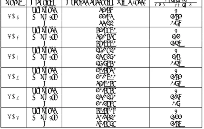
(6) Vol.2012-MPS-87 No.1 2012/3/1. IPSJ SIG Technical Report Table 2. Average execution times of the algorithms on different graphs.. Graph SG0. SG1. SG2. SG3. SG4. SG5. Algorithm Proposed NSGA-II SA Proposed NSGA-II SA Proposed NSGA-II SA Proposed NSGA-II SA Proposed NSGA-II SA Proposed NSGA-II SA. Average execution Time (sec) 32.48 22.83 33.11 42.6570 31.0435 46.7870 19.0510 13.5290 19.9740 27.4630 20.0700 31.7045 20.4545 13.0190 20.1685 47.4808 30.3410 38.4595. P roposed N SGA−II or SA. 1.42 0.98 1.2 1.17 1.4 0.17 1.42 0.97 1.38 0.9 1.22 1.47. 5. Conclusion We have proposed a memory efficient Particle Swarm Optimization (PSO) based algorithm for solving the multi-objective path optimization problem. The proposed algorithm reduces memory requirements by storing the objective function values of the global best and local best positions instead of the particles. Each position is represented by a complete path. The particles change their new positions by modifying the sub-paths in their current positions. The proposed algorithm is executed on an ARM based embedded system. The proposed algorithm is compared with NSGA-II and SA. The comparison results show that the proposed algorithm has found Pareto optimal solutions of quality very close to the NSGA-II and better than SA. The average execution time of the proposed algorithm is also remains within 1.42 times of NSGA-II and 1.47 times of SA. Based on the experimental results, we can conclude that the proposed algorithm is suitable to perform multi-objective path optimization in embedded systems. which generally have less powerful processor and limited memory. In the future, the proposed algorithm will be applied to perform path optimization in the navigation systems of electric vehicles. References 1) Zbigniew TARAPATA, Selected Multicriteria Shortest Path Problems: AN Analysis of Complexity, Models and Adoption of Standard Algorithms, Int. J. Appl. Math. Comput. Sci., Vol. 17, No. 2, (2007) 269-287. 2) M.R. Garey and D. S. Johnson, Computers and Intractability: A Guide to the Theory of NP-Completeness, W. H. Freeman and Co., 1997 3) Kalyanmoy Deb, Amrit Pratap, Sameer Agarwal, and T. Meyarivan, A Fast and Elitist Multiobjective Genetic Algorithm: NSGAII, IEEE Trans. Evolutionary Computation, vol. 6, No. 2, (2002) 182- 197. 4) S.M. Sait & H. Youssef, Iterative Computer Algorithms with Applications in Engineering, IEEE Computer Society Press, 1999. 5) Johannes M. Bader, Hypervolume-Based Search for Multiobjective Optimization: Theory and Methods, Ph.D. dissertation, Swiss Federal Inst. Technology (ETH) Zurich, Switzerland, 2009. 6) J. Kennedy, R. Eberhart, Particle Swarm Optimization, Proceedings of 1995 IEEE International Conference on Neural Network, pp. 1942-1948 (1995). 7) Fabien Viger, Matthieu Latapy, Efficient and simple generation of random simple connected graphs with prescribed degree sequence, 11th Conference of Computing and Combinatoric (COCOON 2005), (2005) 440-449. 8) Carlos M. Fonseca, Lus Paquete, and Manuel Lpez-Ibez, An improved dimension - sweep algorithm for the hypervolume indicator, 2006 IEEE Congress on Evolutionary Computation (CEC’06), (2006) 1157-1163. 9) Hollander, M., and D. A. Wolfe, Nonparametric Statistical Methods, John Wiley & Sons, Inc., 1999. 10) http://www.embeddedarm.com. 6. ⓒ 2012 Information Processing Society of Japan.

(7)