A modified scaling BFGS method for nonconvex minimization

A modified scaling BFGS method for nonconvex

minimization

Kiyohisa Sugasawa and Hiroshi Yabe

(Received March 7, 2013; Revised July 29, 2013)

Abstract In this paper, we propose a modified scaling BFGS method for unconstrained minimization. A remarkable feature of the proposed method is that it can improve the performance of the BFGS method and possesses a global convergence property without convexity assumption on the objective function. Under certain assumptions, we also establish superlinear convergence of the method. Finally we show numerical results.

AMS 2010 Mathematics Subject Classification. 65K05, 90C30, 90C53.

Key words and phrases. Unconstrained minimization, nonconvex optimization,

quasi-Newton method, BFGS method, global convergence, superlinear conver-gence.

§1. Introduction

This paper is concerned with the unconstrained minimization problem min f (x), x∈ Rn,

(1.1)

where f : Rn → R is continuously differentiable. In the following, g(x) and G(x) denote the gradient and Hessian matrix of f at x, respectively. Quasi-Newton methods are effective numerical methods for solving (1.1), and they are iterative methods of the form

xk+1 = xk+ αkdk,

where xk is a current approximation to a solution for (1.1), αk is a step size

and dk is a search direction obtained by solving the linear system of equations

Bkdk =−gk.

Here gkdenotes g(xk) and the matrix Bk is an approximation to Gk≡ G(xk).

The matrix Bk is updated at every iteration by means of a quasi-Newton

updating formula. There are some kinds of updating formulas. In particular, the BFGS formula is one of the most effective formulas and is given by

Bk+1= Bk− BksksTkBk sT_kBksk +yky T k y_kTsk , where sk= xk+1− xk and yk= gk+1− gk.

Throughout this paper, let fk denote f (xk).

The BFGS method is widely used due to its favorable numerical experience and fast convergence property. However, the performance of the conventional BFGS method may be greatly influenced by an unsuitable search direction when the Hessian matrix is ill-conditioned. To overcome this difficulty, sev-eral researchers proposed scaling BFGS methods. For example, Oren and Luenberger [14, 13] suggested a class of the method that they referred to as self-scaling variable metric methods (SSVMs). They multiplied Bk by an

ap-propriate scalar ωk before it was updated, and they used the sized BFGS

updating formula Bk+1= ωk ( Bk− BksksTkBk sT kBksk ) + yky T k yT ksk ,

in which the parameter ωk was chosen as

ωOL_k = y T ksk sT_kBksk , ω_kIOL= y T kBk−1yk y_kTsk ,

which can accelerate the single-step convergence of quasi-Newton methods for a quadratic objective function. Another choice of ωk is given by Al-Baali [2]

as follows ω_kAB = min { y_kTsk sT kBksk , 1 } .

In [2], Al-Baali showed that the sized BFGS method with ω_kAB is competi-tive with the standard BFGS method. Furthermore, other choices of ωk and

numerical results were derived by Al-Baali [1, 2], Nocedal and Yuan [11] and Yabe et al. [16], for example.

More recently, a different scaling BFGS method was derived by Cheng and Li [5]. In order to improve the condition number of the Hessian matrix, they

noticed the following approximate relation γkf (x) (1.2) ≈ γk ( fk+1+ gk+1T (x− xk+1) + 1 2(x− xk+1) T_G k+1(x− xk+1) ) , where γk is some scalar. Differentiating (1.2) and substituting xk into x yield

the relation

γkGk+1sk≈ γkyk,

from which they proposed a new secant condition: Bk+1sk= γkyk.

(1.3)

We call γk the scaling factor in this paper. In [5], they chose the following

scaling factor γ_kCL= y T ksk ∥yk∥2 . (1.4)

Based on (1.3) and (1.4), Bk is updated by

Bk+1= Bk− BksksTkBk sT kBksk + γ_kCLyky T k yT ksk . (1.5)

They called the method based on (1.4) and (1.5) the spectral scaling BFGS method. By using this method, the largest eigenvalue of Bk is strictly less

than Tr(B1)+k. Therefore, the spectral scaling BFGS method has a good

self-correcting property with respect to the trace of Bk. Moreover, they showed the

global convergence of their method for a uniformly convex objective function and good numerical performance in [5]. Yuan [17] also proposed a modified BFGS method.

Besides, several researchers studied another secant condition: Bk+1sk = ˆyk, yˆk = yk+ ϕksk.

(1.6)

Li and Fukushima [9] showed that under some conditions the modified BFGS method based on (1.6) with a nonnegative parameter ϕk has a global

conver-gence property without convexity assumption on the objective function. In addition, they also established superlinear convergence of their method.

In this paper, we study a scaling BFGS method with γkyˆk (We call the modified scaling BFGS method) and obtain the global convergence property without convexity assumption of f . Moreover, we also establish the superlinear convergence of the method. In addition, we apply a new scaling factor to the

method and prove its convergence property.

We organize the paper as follows. In the next section, we propose a modified scaling BFGS method. In Section 3, we prove the global and superlinear convergence of our method. In Section 4, we apply new scaling factors to the method and establish its convergence property. Finally, in Section 5, we present some numerical experiments.

§2. Modified scaling BFGS method

In this section, we propose a modified scaling BFGS method. First, we recall the modification to the standard BFGS method in [9]. Note that if f is twice continuously differentiable, we have the following approximation

Gk+1sk≈ yk,

(2.1)

which yields the secant condition Bk+1sk= yk. So the approximate matrix of Gk+1is usually produced based on (2.1). However, since Gk+1 is not generally

positive definite when f is nonconvex, Bk+1 may not afford a good

approx-imation of Gk+1. To overcome this difficulty, we can replace Gk+1 by the

matrix

¯

Gk+1 ≡ Gk+1+ ϕkI,

where I is the identity matrix and ϕkis chosen so that ¯Gk+1is positive definite.

The matrix ¯Gk+1 will satisfy the following relation

¯

Gk+1sk = (Gk+1+ ϕkI)sk≈ ˆyk,

(2.2)

where ˆyk is defined by (1.6). Li and Fukushima [9] used the modified secant

condition (1.6) based on (2.2).

Following the idea of Cheng and Li [5], we multiply the both sides of (2.2) by a scaling factor γk as follows

γkG¯k+1sk≈ γkyˆk.

This leads to the following secant condition (2.3) Bk+1sk= γkyˆk.

When γk= 1 and ϕk= 0, we get the standard secant condition. An

appropri-ate choice of γk and ϕk may give a scaling BFGS method which has a global

convergence property without convexity assumption of f and good numerical results. In Section 4, we will present several concrete choices of γk and ϕk.

Now, we propose the modified scaling BFGS method (msBFGS) based on (2.3).

[Algorithm of the msBFGS method]

 Step 0. Choose an initial point x0 ∈ Rnand an initial symmetric positive

definite matrix B0 ∈ Rn×n. Choose constants σ1, σ2 and C such that

0 < σ1 < σ2 < 1 and C > 0. Let k:=0.

 Step 1. Solve the following linear system of equations to obtain dk: Bkdk=−gk.

 Step 2. Find a step size αk satisfying the Wolfe conditions: f (xk+ αkdk)≤ f(xk) + σ1αkgTkdk,

(2.4)

g(xk+ αkdk)Tdk ≥ σ2gkTdk.

(2.5)

 Step 3. Let the next iterate be xk+1 = xk+ αkdk.

 Step 4. If the stopping condition is satisfied, then stop. Otherwise go to Step5

 Step 5. Give γk > 0 and ϕk∈ [0, C]. Let ˆyk= yk+ ϕksk.

 Step 6. Update Bk by using the msBFGS formula Bk+1 = Bk− BksksTkBk sT_kBksk + γk ˆ ykyˆTk ˆ y_kTsk . (2.6)

 Step 7. Let k := k + 1 and go to Step 1.

It follows from γk> 0, ϕk≥ 0 and (2.5) that for any k γkyˆkTsk ≥ γkykTsk> 0.

(2.7)

Therefore, the matrix Bk+1is positive definite as long as Bkis positive definite.

Consequently, dk becomes a descent search direction of f at xk.

§3. Convergence analysis

In this section, we will establish the global and superlinear convergence prop-erty of the msBFGS method. To this end, we make the following assumptions.

Assumption A

(1) The level set at the initial point x0

Ω ={x ∈ Rn | f(x) ≤ f(x0)}

is bounded.

(2) The objective function f is continuously differentiable in an open convex set containing Ω, and there exists a positive constant Lg such that

∥g(x) − g(y)∥ ≤ Lg∥x − y∥ for all x, y ∈ Ω.

Now we analyze convergence properties of our method. The global convergence is proved in Section 3.1, and the local and superlinear convergence is shown in Section 3.2.

In the remainder of this paper, let

cos θk = sT_kBksk ∥sk∥∥Bksk∥ , (3.1) qk = sT_kBksk ∥sk∥2 , (3.2) Ψ(Bk) = Tr(Bk)− ln(detBk) and zk= γkyˆk. (3.3)

Note that Ψ(Bk) can be represented by the expression

(3.4) Ψ(Bk) =

n

∑

i=1

(µk,j− ln µk,j),

where 0 < µk,1≤ · · · ≤ µk,n are the eigenvalues of Bk. We also note that the

function

w(p) = p− ln(p), p > 0

is strictly convex and has the minimum value of 1 at p = 1. Therefore, Ψ(Bk)≥ n holds. Taking the trace in the msBFGS formula, we get

Tr(Bk+1) = Tr(Bk)−∥Bk sk∥2 sT_kBksk + ∥zk∥ 2 zT_ksk .

Furthermore, taking the determinant in the msBFGS formula, we have det(Bk+1) = det ( Bk ( I−sks T kBk sT kBksk +B −1 k zkzkT zT ksk )) = det(Bk) ( 1− s T k sT kBksk Bksk ) ( 1 +(B −1 k zk)T zT ksk zk ) − det(Bk) ( −zT ksk sT kBksk ) ( sT_kBkB_k−1zk zT ksk ) = det(Bk) z_kTsk sT kBksk ,

where the second equality can be found in Lemma 7.6 of [7]. Therefore, we derive the following expression for Ψ(Bk).

Ψ(Bk+1) = Ψ(Bk)−∥Bk sk∥2 sT_kBksk +∥zk∥ 2 z_kTsk − ln ( z_kTsk sT_kBksk ) = Ψ(Bk)− ( ∥Bksk∥∥sk∥ sT_kBksk )2 sT_kBksk ∥sk∥2 +∥zk∥ 2 z_kTsk − ln ( z_kTsk ∥sk∥2 ∥sk∥2 sT_kBksk ) .

Using the definitions (3.1) and (3.2), we have

Ψ(Bk+1) = Ψ(Bk) +∥zk∥ 2 zT ksk − ln zkTsk ∥sk∥2 − qk cos2_θ k + ln qk (3.5) = Ψ(Bk) +∥zk∥ 2 zT_ksk − ln zkTsk ∥sk∥2 + ln cos2θk− 1 + ( 1− qk cos2_θ k + ln qk cos2_θ k ) . 3.1. Global convergence

To prove the global convergence, we first introduce the following general result (see Theorem 3.2 of [12]).

Lemma 3.1. Suppose that Assumption A holds. Consider any iterative method

of the form xk+1 = xk+ αkdk, where a search direction dk satisfies the descent condition gT_kdk< 0 and a step size αk satisfies the Wolfe conditions (2.4) and

(2.5). Then the following Zoutendijk condition holds (3.6) ∞ ∑ k=0 (gT kdk)2 ∥dk∥2 <∞.

The next lemma gives the conditions on γkand ϕk and is useful in showing

the global convergence.

Lemma 3.2. Let B0 be symmetric positive definite and Bk be updated by

(2.6). Suppose that there exist positive constants m, M and t1 such that for

any k≥ t1, γk and ϕk satisfy

γk(ρ(1)_k + ϕk) ≥ m, (3.7) γk(ρ(2)_k + 2ϕkρ(1)_k + ϕ2k) ≤ M(ρ (1) k + ϕk), (3.8) where ρ(1)_k = yTksk ∥sk∥2 and ρ (2) k = ∥y k∥2

∥sk∥2. Then there exist positive constants

β0, β1, β2 and β3 such that for any positive integer k (≥ t1), the following

inequalities cos θj ≥ β0, (3.9) ∥Bjsj∥ ≤ β1∥sj∥, (3.10) β2∥sj∥2 ≤ sTjBjsj ≤ β3∥sj∥2 (3.11)

hold at least ⌈(k − t1+ 1)/2⌉ values of j ∈ {t1, . . . , k}.

Proof. We can prove this lemma similarly to the proof of Theorem 2.1 in [4]. We first note that ρ(1)_k + ϕk= ˆ yT ksk ∥sk∥2 (3.12) and ρ(2)_k + 2ϕkρ (1) k + ϕ2k ρ(1)_k + ϕk = ∥yk∥ 2_{+ 2ϕ} kyTksk+ ϕ2k∥sk∥2 yT ksk+ ϕk∥sk∥2 = ∥ˆyk∥ 2 ˆ yT ksk . (3.13)

From (3.3), (3.7), (3.8), (3.12) and (3.13), we have z_kTsk ∥sk∥2 = γk ˆ yT_ksk ∥sk∥2 = γk(ρ(1)k + ϕk)≥ m and ∥zk∥2 z_kTsk = γk∥ˆyk∥ 2 sT_kyˆk = γk ρ(2)_k + 2ϕkρ(1)k + ϕ2k ρ(1)_k + ϕk ≤ M.

Thus, it follows from (3.5) that Ψ(Bk+1)≤ Ψ(Bk) + M − ln m + ln cos2θk− 1 + ( 1− qk cos2_θ k + ln qk cos2_θ k ) ≤ . . . ≤ Ψ(Bt1) + (M− ln m − 1)(k − t1+ 1) + k ∑ j=t1 ( ln cos2θj+ ( 1− qj cos2_θ j + ln qj cos2_θ j )) . Let us define ηj by ηj =− ln cos2θj− ( 1− qj cos2_θ j + ln qj cos2_θ j ) . (3.14) The function u(p) = 1− p + ln p (3.15)

achieves the maximum value of 0 at p = 1. Thus, ηj ≥ 0 holds. Furthermore,

since Ψ(Bk+1) > 0, we have 1 k− t1+ 1 k ∑ j=t1 ηj < Ψ(Bt1) k− t1+ 1 + (M− 1 − ln m). (3.16)

Let us now define Jkto be a set consisting of the

⌈ k−t1+1 2 ⌉ indices correspond-ing to the ⌈ k−t1+1 2 ⌉

smallest values of ηj for t1 ≤ j ≤ k, and let ηmk denote

the largest value of ηj for j∈ Jk. Then

1 k− t1+ 1 k ∑ j=t1 ηj = 1 k− t1+ 1  ∑ j∈Jk ηj+ ∑ j̸∈Jk ηj   ≥ 1 k− t1+ 1  η_mk+∑ j̸∈Jk ηmk   ≥ 1 k− t1+ 1 ( ηmk+ ηmk ( k− t1+ 1− ⌈ k− t1+ 1 2 ⌉)) ≥ ηmk k− t1+ 1 + ηmk k− t1+ 1 ( k− t1+ 1− ( k− t1+ 1 2 + 1 )) = ηmk 2 .

Thus, from (3.16), we have that, for all j∈ Jk, ηj < 2 (Ψ(Bt1) + M− 1 − ln m) ≡ β

′

0.

(3.17)

Since the term inside brackets in (3.14) is less than or equal to zero, we con-clude from (3.14) and (3.17) that for all j∈ Jk

− ln cos2_θ j < β ′ 0. Therefore, we obtain cos θj > e−β ′ 0/2≡ β_0,

which implies (3.9). Similarly, from (3.14) and (3.17), we have that for all j∈ Jk, 1− qj cos2_θ j + ln qj cos2_θ j >−β₀′.

Note also that the function (3.15) achieves the maximum value of 0 at p = 1 and satisfies u(p)→ −∞ both as p → 0 and p → ∞. Therefore, it follows that for all j∈ Jk

0 < β₂′ ≤ qj cos2_θ

j ≤ β3

for positive constants β₂′ and β3. Therefore, we obtain

qj ≤ β3cos2θj ≤ β3, qj ≥ β ′ 2cos2θj ≥ β ′ 2β20 ≡ β2

from which we get by using (3.2)

β2≤

sT jBjsj ∥sj∥2 ≤ β

3,

which implies (3.11). Finally, since ∥Bjsj∥ ∥sj∥ = qj cos θj , we have for j∈ Jk ∥Bjsj∥ ∥sj∥ ≤ β3 β0 ≡ β1 . Therefore, the proof is complete.

By (3.12) and (3.13), we note that (3.7) and (3.8) equal γk ˆ yT_ksk ∥sk∥2 ≥ m and γk ∥ˆyk∥2 sT kyˆk ≤ M.

The following theorem shows the global convergence of the msBFGS method.

Theorem 3.3. Let {xk} be the infinite sequence generated by the msBFGS method. Suppose that Assumption A holds. If (3.7) and (3.8) are satisfied for any k≥ 0, then

lim inf

k→∞ ∥gk∥ = 0.

Proof. Let K ={k|Inequalities (3.9), (3.10) and (3.11) hold}. Since Lemma 3.2 holds for the case t1= 0, the set K is not empty. For the msBFGS method,

Lemma 3.1 holds and the Zoutendijk condition can be written as

∞ ∑ k=0 (∥gk∥ cos θk)2<∞. Therefore, by (3.9), we obtain lim k→∞, k∈K∥gk∥ = 0,

which implies the result.

Theorem 3.3 yields the following corollary that corresponds to the conver-gence result of Cheng and Li [5].

Corollary 3.4. Suppose that Assumption A and the following two

assump-tions hold.

(1) The objective function f is twice continuously differentiable.

(2) The level set Ω is convex and there exist positive constants λ1 and λ2

such that

λ1∥v∥2 ≤ vTG(x)v≤ λ2∥v∥2 ∀x ∈ Ω, v ∈ Rn.

Let γk = yT

ksk

∥yk∥2, ϕk = 0 and {xk} be the infinite sequence generated by the

msBFGS method. Then

lim inf

3.2. Superlinear convergence

Now we turn to prove the superlinear convergence of the msBFGS method. To do this, we make the following additional assumptions.

Assumption B

(1) The function f is twice continuously differentiable in an open convex neigh-borhood U (x∗) of x∗, where g(x∗) = 0 and G(x∗) is positive definite.

(2) The second derivative G is Lipschitz continuous in U (x∗), i.e. there exists a constant LG> 0 such that

∥G(x) − G(x∗_{)∥ ≤ L}

G∥x − x∗∥

(3.18)

holds for any x in U (x∗). (3){xk} converges to x∗.

(4) There exist positive constants c1 and c2 such that c1 ≤ γk ≤ c2 holds for

any k.

Under Assumption B(1), G(x) is uniformly positive definite for any x∈ U(x∗). Therefore, there is a constant m′ > 0 such that for all x∈ U(x∗)

∥g(x)∥ ≥ m′∥x − x∗∥ (3.19)

and

vTG(x)v≥ m′∥v∥2 ∀v ∈ Rn. (3.20)

Particularly, by using the mean-value theorem, these show that for k≥ k0

yT_ksk= (∫ 1 0 G(xk+ tsk)skdt )T sk ≥ m′∥sk∥2,

since xk + tsk ∈ U(x∗) for k ≥ k0, where k0 is some nonnegative integer.

Therefore, under Assumptions A and B, (3.12) and (3.13) yield that γk(ρ(1)k + ϕk) = γk ˆ yT_ksk ∥sk∥2 = γk ( yT ksk ∥sk∥2 + ϕk ) ≥ γk ( m′∥sk∥2 ∥sk∥2 + ϕk ) ≥ γk(m′+ ϕk) ≥ γkm′ ≥ c1m′

and γk(ρ (2) k + 2ϕkρ (1) k + ϕ2k) ρ(1)_k + ϕk = γk∥ˆyk∥ 2 ˆ y_kTsk ≤ γk (Lg+ ϕk)2∥sk∥2 m′∥sk∥2 ≤ c2 (Lg+ ϕk)2 m′ .

These imply that inequalities (3.7) and (3.8) hold for m = c1m′, M = c2(Lg+C) 2

m′

and t1 = k0. Thus, there exists a nonempty set Jk = {j|Inequalities (3.9),

(3.10) and (3.11) hold, k0≤ j ≤ k} from Lemma 3.2. Lemma 3.5. Under Assumptions A and B, we have

∞ ∑ k=0 ∥xk− x∗∥ < ∞ (3.21) and ∞ ∑ k=0 τk<∞, (3.22) where τk= max{∥xk− x∗∥, ∥xk+1− x∗∥}.

Proof. We can assume k≥ k0 without loss of generality. It follows from (2.5)

that

−(1 − σ2)gkTsk≤ (gk+1− gk)Tsk≤ ∥gk+1− gk∥∥sk∥ ≤ Lg∥sk∥2.

Using (3.1) yields the relation (1− σ2)

Lg ∥gk∥ cos θk≤ ∥sk∥.

(3.23)

Since f is convex function on U (x∗), we have fk− f∗ ≤ gTk(xk− x∗)

≤ ∥gk∥∥xk− x∗∥ ≤ ∥gk∥2

m′ , (3.24)

where the last inequality follows from (3.19). For j∈ Jk, we obtain from (2.4), (3.1) and (3.23) fj+1 ≤ fj+ σ1gTjsj = fj− σ1∥gj∥∥sj∥ cos θj ≤ fj− σ1 1− σ2 Lg ∥gj∥ 2_{cos θ} j2. Therefore, by (3.9), we have fj− fj+1 ≥ σ1β02 1− σ2 Lg ∥gj∥ 2_. (3.25)

Letting η≡ σ1β20(1− σ2)/Lg, we obtain from (3.24) and (3.25) m′(fj− f∗) ≤

1

η(fj− fj+1), which implies

fj+1− f∗ ≤ r2(fj− f∗),

where r ≡√1− ηm′. (Note that 1 > 1− ηm′ ≥ 0 since {fk} is a decreasing

sequence.) Since Jk has at least⌈(k − k0+ 1)/2⌉ elements by Lemma 3.2 and

{fk} is decreasing, we have fk+1− f∗ ≤ (fjk

max+1− f∗) (j

k

max ≡ arg max{j|j ∈ Jk}) ≤ r2_(f jk max − f∗) ≤ . . . ≤ r2⌈(k−k0+1)/2⌉−1_(f jk min− f∗) (j k

min≡ arg min{j|j ∈ Jk}) ≤ r2(k−k0+1)/2−1_(f jk min− f∗) = rk−k0_(f jk min− f∗) ≤ rk−k0_(f k0 − f∗).

Moreover, we can derive the lower bound of fk+1− f∗ from Taylor’s expansion

and (3.20) as follows 1 2m ′_∥x k+1− x∗∥2 ≤ fk+1− f∗. Therefore, we obtain ∥xk+1− x∗∥ ≤ √ 2(fk+1− f∗) m′ ≤ √ 2(fk0 − f∗)r k m′rk0 = a1 (√ r )k ,

where a1 ≡

√

2(f_k0−f_∗)

m′rk0 . Hence we obtain (3.21). Finally, since τk ≤ ∥xk− x∗∥ + ∥xk+1− x∗∥, (3.22) follows from (3.21) directly.

Now, we add the following assumption.

Assumption C

The parameters γk and ϕk satisfy ∞ ∑ k=0 |γk− 1| < ∞ and ∞ ∑ k=0 ϕk<∞. (3.26)

Adding Assumption C, we have the following lemma.

Lemma 3.6. Suppose that Assumptions A, B and C hold. Then there exists

a sequence{ϵk} such that {sk} and {zk} satisfy for k sufficiently large ∥γkyˆk− G(x∗)sk∥ ∥sk∥ ≤ ϵk , (3.27) and ∑∞ k=0 ϵk<∞ holds. Proof. Using (3.18), we have

∥γkyˆk− G(x∗)sk∥ ≤ ∥(γk− 1)ˆyk∥ + ∥yk+ ϕksk− G(x∗)sk∥ ≤| γk− 1 | ∥ˆyk∥ + ∫ 1 0 ∥G(xk+ tsk)− G(x∗)∥dt∥sk∥ + ∥ϕksk∥ ≤| γk− 1 | ∥ˆyk∥ + ∫ 1 0 ∥xk+ tsk− x∗∥dtLG∥sk∥ + ∥ϕksk∥ ≤| γk− 1 | ∥ˆyk∥ + ∫ 1 0 (∥t(xk+1− x∗)∥ + ∥(1 − t)(xk− x∗)∥)dtLG∥sk∥ +∥ϕksk∥ =| γk− 1 | ∥ˆyk∥ + 1 2(∥xk+1− x ∗_{∥ + ∥x} k− x∗∥) LG∥sk∥ + ∥ϕksk∥ ≤| γk− 1 | ∥ˆyk∥ + max{∥xk+1− x∗∥, ∥xk− x∗∥}LG∥sk∥ + ∥ϕksk∥ ≤| γk− 1 | (∥yk∥ + ∥ϕksk∥) + (LGτk+ ϕk)∥sk∥ ≤ (| γk− 1 | (Lg+ ϕk) + LGτk+ ϕk)∥sk∥.

Therefore, (3.27) holds for ϵk =| γk−1 | (Lg+ ϕk) + LGτk+ ϕk, and ∞

∑

k=0

ϵk<∞

Moreover, we give the following lemma to show the convergence property. This lemma was shown by Dennis and Mor´e [6].

Lemma 3.7. Let f : Rn → R be twice differentiable in an open convex set

D in Rn, and assume that for some ˆx in D, G is continuous at ˆx and G(ˆx) is nonsingular. Let {Bk} in Rn×n be a sequence of nonsingular matrices and suppose that for some x0 in D, the sequence {xk} generated by

xk+1= xk− B_k−1gk

remains in D and converges to ˆx. Then the sequence {xk} converges Q-superlinearly to ˆx and g(ˆx) = 0 if and only if

lim k→∞ ∥(Bk− G(ˆx))(xk+1− xk)∥ ∥xk+1− xk∥ = 0. (3.28)

Note that (3.28) is called the Dennis-Mor´e condition. From Lemma 3.7, we obtain the next theorem.

Theorem 3.8. Let the sequences{xk} and {Bk} be generated by the msBFGS method. Suppose that Assumptions A, B and C hold. Then

lim k→∞ ∥(Bk− G(x∗))sk∥ ∥sk∥ = 0 (3.29)

holds and the sequence{∥B−1_k ∥} is bounded. Moreover, if the parameter σ1 in

(2.4) is chosen to satisfy σ1 ∈

(

0,1₂), then the sequence {xk} converges to x∗ superlinealy.

Proof. Let us define ˜ sk= G(x∗) 1 2s_k, z˜_k= G(x∗)− 1 2z_k, (3.30) ˜ Bk= G(x∗)− 1 2B_kG(x∗)− 1 2, (3.31) cos ˜θk= ˜ sT kB˜ks˜k ∥ ˜Bks˜k∥∥˜sk∥ and ˜ qk= ˜ sT_kB˜ks˜k ∥˜sk∥2 .

Though the first part of this theorem can be shown in the same way as the proof of Theorem 3.2 in [4], we do not omit the proof for readability. From (2.6), (3.30) and (3.31), it follows that

˜ Bk+1 = ˜Bk− ˜ Bks˜ks˜TkB˜k ˜ sT_kB˜k˜sk + z˜kz˜ T k ˜ zT ks˜k .

Thus, we obtain, just as in (3.5) Ψ( ˜Bk+1) = Ψ( ˜Bk) + ∥˜zk∥ 2 ˜ sT kz˜k − ln s˜Tkz˜k ∥˜sk∥2 + ln cos2θ˜k− 1 (3.32) + ( 1− q˜k cos2_θ˜ k + ln q˜k cos2_θ˜ k ) . For k sufficiently large, it follows from (3.27) that

∥˜zk− ˜sk∥ = ∥G(x∗)− 1 2z_k− G(x∗) 1 2s_k∥ (3.33) ≤ ∥G(x∗₎−1 2∥∥γ_kyˆ_k− G(x∗)s_k∥ ≤ ∥G(x∗)−12∥ϵ_k∥s_k∥ = ∥G(x∗)−12∥ϵ_k∥G(x∗)− 1 2G(x∗) 1 2s_k∥ ≤ ∥G(x∗)−12∥2ϵ_k∥˜s_k∥ = ¯cϵk∥˜sk∥,

where ¯c =∥G(x∗)−12∥2. Using the triangle inequality yields

∥˜zk− ˜sk∥ ≥ ∥˜zk∥ − ∥˜sk∥ and ∥˜zk− ˜sk∥ = ∥˜sk− ˜zk∥ ≥ ∥˜sk∥ − ∥˜zk∥. So we have (1− ¯cϵk)∥˜sk∥ ≤ ∥˜zk∥ ≤ (1 + ¯cϵk)∥˜sk∥. (3.34)

From (3.33) and (3.34), it follows that

∥˜zk∥2− 2˜zTks˜k+∥˜sk∥2 ≤ ¯c2ϵ2k∥˜sk∥2

and

(1− ¯cϵk)2∥˜sk∥2− 2˜zkT˜sk+∥˜sk∥2≤ ∥˜zk∥2− 2˜zkT˜sk+∥˜sk∥2,

from which we get

(1− ¯cϵk)2∥˜sk∥2− 2˜zkT˜sk+∥˜sk∥2≤ ¯c2ϵ2k∥˜sk∥2. (3.35) By (3.35), we have ˜ z_kT˜sk ∥˜sk∥2 ≥ 1 − ¯cϵk . (3.36)

Since ˜z_kT˜sk > 0 is satisfied, (3.34) yields ∥˜zk∥2 ˜ zT k˜sk ≤ (1 + ¯cϵk)2∥˜sk∥ 2 ˜ zT ks˜k . (3.37)

By using the fact ∑∞_k=0ϵk <∞, there exists an integer ¯k such that ¯cϵk ≤ 1₂

for k≥ ¯k. Therefore, it follows from (3.36) and (3.37) for k ≥ ¯k that ∥˜zk∥2 ˜ z_kT˜sk ≤ (1 + ¯cϵ k)2∥˜sk∥ 2 ˜ z_kTs˜k (3.38) ≤ (1 + ¯cϵk) 1 + ¯cϵk 1− ¯cϵk = 1 + ϵk ( 2¯c 1− ¯cϵk + ¯c + 2¯c 2_ϵ k 1− ¯cϵk ) ≤ 1 + ϵk ( 2¯c 1−1₂ + ¯c + 2¯c1₂ 1− 1₂ ) = 1 + 7¯cϵk.

We notice that the inequality − ln(1 − x) ≤ 2x holds for 0 < x ≤ 1₂. So it follows from (3.36)

− ln z˜kTs˜k

∥˜sk∥2 ≤ − ln(1 − ¯cϵk

)≤ 2¯cϵk.

(3.39)

Thus, by (3.32), (3.38) and (3.39), for k≥ ¯k we have Ψ( ˜Bk+1)≤ Ψ( ˜Bk) + 9¯cϵk+ ln cos2θ˜k+ ( 1− q˜k cos2_θ˜_k + ln ˜ qk cos2_θ˜_k ) . Hence by using (3.32) again, there is a positive constant ˆc such that

Ψ( ˜Bk+1) (3.40) ≤ Ψ( ˜B_k¯) + k ∑ j=¯k ( 9¯cϵj+ ln cos2θ˜j+ ( 1− q˜j cos2_θ˜ j + ln q˜j cos2_θ˜ j )) = Ψ( ˜B_k¯₋₁) + ∥˜z ¯ k−1∥2 ˜ sT ¯ k−1z˜¯k−1 − lns˜ T ¯ k−1z˜¯k−1 ∥˜s_k¯₋₁∥2 + ln cos2θ˜¯_k−1− 1 + ( 1− q˜k−1¯ cos2_θ˜_¯ k−1 + ln q˜¯k−1 cos2_θ˜_¯ k−1 ) + k ∑ j=¯k ( 9¯cϵj+ ln cos2θ˜j + ( 1− q˜j cos2_θ˜ j + ln q˜j cos2_θ˜ j ))

= Ψ( ˜B¯_k−1) + k ∑ j=¯k−1 ( ln cos2θ˜j+ 1− ˜ qj cos2_θ˜_j + ln ˜ qj cos2_θ˜_j + 9¯cϵj ) + ¯ k−1 ∑ j=¯k−1 ( −9¯cϵj+ ∥˜zj∥ 2 ˜ sT jz˜j − ln s˜ T jz˜j ∥˜sj∥2 − 1 ) = Ψ( ˜B¯_k−2) + k ∑ j=¯k−2 ( ln cos2θ˜j+ 1− ˜ qj cos2_θ˜_j + ln ˜ qj cos2_θ˜_j + 9¯cϵj ) + ¯ k−1 ∑ j=¯k−2 ( −9¯cϵj+ ∥˜zj∥ 2 ˜ sT jz˜j − ln s˜ T jz˜j ∥˜sj∥2 − 1 ) = . . . = Ψ( ˜B0) + k ∑ j=0 ( ln cos2θ˜j+ 1− ˜ qj cos2_θ˜_j + ln ˜ qj cos2_θ˜_j + 9¯cϵj ) + ¯ k−1 ∑ j=0 ( −9¯cϵj+∥˜zj∥ 2 ˜ sT jz˜j − ln s˜ T jz˜j ∥˜sj∥2 − 1 ) = Ψ( ˜B0) + k ∑ j=0 ( ln cos2θ˜j+ 1− ˜ qj cos2_θ˜ j + ln q˜j cos2_θ˜ j + 9¯cϵj ) + ˆc.

Furthermore, similar comments to those for (3.4) and (3.15) indicate Ψ( ˜Bk+1)≥ n and 1 − ˜ qj cos2_θ˜ j + ln q˜j cos2_θ˜ j ≤ 0. (3.41)

From (3.40), (3.41), the expressions ln cos2θ˜j ≤ 0 and

∑_∞

k=0ϵk < ∞, we see

that{Ψ( ˜Bk)} is bounded, and since

n− k ∑ j=0 ( ln cos2θ˜j + 1− ˜ qj cos2_θ˜ j + ln q˜j cos2_θ˜ j ) ≤ Ψ( ˜B0) + k ∑ j=0 9¯cϵj+ ˆc, we have 0≤ − k ∑ j=0 ( ln cos2θ˜j+ 1− ˜ qj cos2_θ˜ j + ln q˜j cos2_θ˜ j ) <∞. So we obtain ln cos ˜θk→ 0 (3.42)

and 1− q˜k cos2_θ˜_k + ln ˜ qk cos2_θ˜_k → 0. (3.43) Expression (3.42) implies cos ˜θk → 1. (3.44)

Furthermore, since (3.43) and the comments following (3.15) show q˜k

cos2_θ˜ k → 1, (3.44) implies ˜ qk→ 1. (3.45)

Now it follows from (3.44) and (3.45) that ∥(Bk− G(x∗))sk∥2 ∥sk∥2 1 ∥G(x∗₎1 2∥4 ≤ ∥(Bk− G(x∗))sk∥2 ∥G(x∗₎1 2s_k∥2∥G(x∗) 1 2∥2 ≤ ∥G(x∗)− 1 2(B_k− G(x∗))s_k∥2 ∥G(x∗₎1 2s_k∥2 = ∥( ˜Bk− I)˜sk∥ 2 ∥˜sk∥2 = ∥ ˜Bks˜k∥ 2_{− 2˜s}T kB˜k˜sk+∥˜sk∥2 ∥˜sk∥2 = q˜ 2 k cos2_θ˜ k − 2˜qk+ 1→ 0,

which implies (3.29). Since{Ψ( ˜Bk)} is bounded, (3.4) implies that there is a

positive constant P such that for all k P ≥

n

∑

j=1

(˜µk,j− ln ˜µk,j) > 0,

where 0 < ˜µk,1 ≤ · · · ≤ ˜µk,n are the eigenvalues of ˜Bk. Since this means P ≥ ˜µk,j− ln ˜µk,j > 0 for all 1≤ j ≤ n, there exist positive constants p1 and

p2 such that

p1≤ ˜µk,j≤ p2 for all 1≤ j ≤ n,

where p1 and p2 satisfy p1− ln p1= P and p2− ln p2 = P . So we get

∥ ˜B_k−1∥2 = √ ρ( ˜B−T_k B˜−1_k ) = √ ρ ( ( ˜B_k−1)2)₌ 1 ˜ µk,1 ≤ 1 p1 ,

where ρ(A) denotes the spectral radius of the matrix A. Therefore, the upper bound of∥B_k−1∥ is estimated by ∥Bk−1∥ = ∥G(x∗)− 1 2G(x∗) 1 2B−1 k G(x∗) 1 2G(x∗)− 1 2∥ ≤ ∥G(x∗₎−1 2∥2∥(G(x∗)− 1 2B_kG(x∗)− 1 2)−1∥ ≤ ∥G(x∗)−12∥2∥ ˜B−1 k ∥.

Next we verify that αk = 1 is accepted for all k sufficiently large. Since ∥dk∥ = ∥Bk−1gk∥ ≤ ∥Bk−1∥∥gk∥ → 0 from the boundedness of ∥Bk−1∥ and

Assumptions B(1) and B(3), by Taylor’s expansion we obtain f (xk+ dk)− f(xk)− σ1gkTdk = (1− σ1)gTkdk+ 1 2d T kG(xk+ tdk)dk = −(1 − σ1)dTkBkdk+ 1 2d T kG(xk+ tdk)dk = − ( 1 2 − σ1 ) dT_kG(x∗)dk+ o(∥dk∥2),

where t∈ (0, 1) and the last equality follows from (3.29). Thus, f(xk+ dk)− f (xk)− σ1g_kTdk ≤ 0 is satisfied for all k sufficiently large. This means that αk= 1 satisfies (2.4) for all k sufficiently large. On the other hand, we have

g(xk+ dk)Tdk− σ2gTkdk = (g(xk+ dk)− gk)Tdk+ (1− σ2)gTkdk

= dT_kG(xk+ tdk)dk− (1 − σ2)dTkBkdk

= σ2dTkG(x∗)dk+ o(∥dk∥2),

where t∈ (0, 1). Thus, we have g(xk+ dk)Tdk ≥ σ2gT_kdk, which means that αk = 1 satisfies (2.5) for all k sufficiently large. From Lemma 3.7 and (3.29),

we can deduce that the sequence{xk} converges superlinearly to x∗.

§4. Practical choices of γk

In this section, we propose three kinds of scaling factors for the msBFGS method and show the convergence properties with them, respectively. The convergence properties of the msBFGS method depend on the choices of γk

and ϕk. For the global convergence, it is important to choose γk and ϕk that

satisfy (3.7) and (3.8), and for the superlinear convergence, it is important to choose them that satisfy (3.26). Li and Fukushima [9] suggested that one of suitable choices of ϕk for the msBFGS method with γk= 1 is

ϕk= δk∥gk∥,

where δk ∈ [δ, ¯δ] (δ and ¯δ are positive constants). This choice may be also

efficient for the convergence properties of the msBFGS method with γk ̸= 1.

Therefore, we choose ϕk in (4.1).

Now, we propose three kinds of scaling factors as follows:

(i) Let Dk be some scaling matrix for ¯Gk. Then, we expect that the

ms-BFGS method with Bkwhich approximates to DkG¯khas a numerical stability.

Such Dk must be the matrix which is a rough approximation to ¯G−1_k . Thus,

we require the relation Dk+1yˆk ≈ sk. Let Dk+1 = γkI for simplicity. By

minimizing the norms ∥sk− γkyˆk∥ and ∥_γ1_ksk− ˆyk∥, we have

γ_k(1) = yˆ T ksk ∥ˆyk∥2 and γ_k(2)= ∥sk∥ 2 ˆ yT ksk ,

respectively. Now, we propose the first scaling factor by using the convex combination of γ_k(1) and γ_k(2) as follows

γk= (1− t)γ(1)k + tγ

(2)

k ,

(4.2)

where t ∈ [0, 1]. If the Wolfe conditions (2.4) and (2.5) are satisfied, then ˆ

yT_ksk > 0 holds. Thus, γk in (4.2) is always positive, which implies that the

msBFGS method with (4.1) and (4.2) generates a descent search direction. For the msBFGS method with (4.1) and (4.2), we obtain the following convergence theorem.

Theorem 4.1. Let ϕk and γk be defined by (4.1) and (4.2), respectively. Let {xk} be the infinite sequence generated by the msBFGS method. Suppose that Assumption A holds. Then

lim inf

k→∞ ∥gk∥ = 0.

Proof. To prove this theorem by contradiction, we assume that there is a con-stant ε > 0 such that∥gk∥ ≥ ε for all k. Since dkis a descent search direction

and (2.4) is satisfied, we have xk∈ Ω for all k. Thus, from Assumption A, ∥gk∥

is bounded above. Therefore, ϕk(= δk∥gk∥) is included in a bounded interval

[0, C] for some C > 0. We note that

ˆ

y_kTsk = ykTsk+ ϕk∥sk∥2 ≥ ϕk∥sk∥2 = δk∥gk∥∥sk∥2 ≥ δε∥sk∥2.

From (3.12) and (4.3), we have γk(ρ (1) k + ϕk) = γk ˆ yT ksk ∥sk∥2 = (1− t) (ˆy T ksk)2 ∥ˆyk∥2∥sk∥2 + t ≥ (1 − t) (δε∥sk∥2)2 (Lg+ C)2∥sk∥4 + t ≥ (1 − t) (δε)2 (Lg+ C)2 + t ≥ min { (δε)2 (Lg+ C)2 , 1 }

and by (3.13) and (4.3), we obtain γk(ρ(2)k + 2ϕkρ(1)k + ϕ2k) ρ(1)_k + ϕk = γk∥ˆyk∥ 2 ˆ y_kTsk = (1− t) + t∥sk∥ 2_∥ˆy k∥2 (ˆyT_ksk)2 ≤ (1 − t) + t(Lg+ C)2∥sk∥4 (δε)2_∥s k∥4 ≤ (1 − t) + t(Lg+ C)2 (δε)2 ≤ max { 1,(Lg+ C) 2 (δε)2 } .

These imply that inequalities (3.7) and (3.8) hold with m = min { (δε)2 (Lg+C)2, 1 } and M = max { 1,(Lg+C)2 (δε)2 }

for any k ≥ 0. Thus, it follows from Theorem 3.3 that lim infk→∞∥gk∥ = 0, which yields a contradiction. Therefore, the

theorem is proved.

(ii) Next, we give another scaling factor. Powell [15] indicated that the BFGS method suffers more from large eigenvalues of Bkthan from small ones

(see also [16]). Thus, we choose

γ_k′ = ( −l + ∥Bksk∥2 sT kBksk ) ˆ yT_ksk ∥ˆyk∥2 , (4.4)

with γ′_k, we have Tr(Bk+1) = Tr(Bk)−∥Bk sk∥2 sT kBksk + γ′_k∥ˆyk∥ 2 ˆ yT ksk = Tr(Bk)− l.

This equality shows that the msBFGS update with γ_k′ can decrease the sum of eigenvalues by −l. Thus, this choice may influence the performance well. However, we can not obtain the convergence property of the msBFGS method with γ′_kand ϕkin (4.1) by using Theorem 3.3. Hence, for given ϕk, we propose

the modified version of (4.4)

γk =                γ_k′ if γ_k′(ρ(1)_k + ϕk)≥ m and γ_k′(ρ(2)_k + 2ϕkρ(1)_k + ϕ2k)≤ ¯M (ρ (1) k + ϕk), 1 otherwise, (4.5)

where m and ¯M are positive constants. If the Wolfe conditions are satisfied, then ρ(1)_k ≥ 0 holds and then γk in (4.5) is always positive. Therefore, the

msBFGS method with (4.1) and (4.5) generates a descent search direction. The following theorem shows the global convergence of the msBFGS method with (4.1) and (4.5).

Theorem 4.2. Let ϕk and γk be defined by (4.1) and (4.5), respectively. Let {xk} be the infinite sequence generated by the msBFGS method. Suppose that Assumption A holds. Then

lim inf

k→∞ ∥gk∥ = 0.

Proof. To prove this theorem by contradiction, we assume that there is a constant ε > 0 such that ∥gk∥ ≥ ε for all k. For the case γk= 1, expressions

(3.12) and (4.3) yield

γk(ρ(1)_k + ϕk) =

ˆ y_kTsk ∥sk∥2 ≥ δε

and equation (3.13) implies

γk(ρ(2)_k + 2ϕkρ(1)_k + ϕ2_k) ρ(1)_k + ϕk = ∥ˆyk∥ 2 ˆ yT ksk ≤ (Lg+ C)2∥sk∥2 δε∥sk∥2 = (Lg+ C) 2 δε .

Thus, these imply that inequalities (3.7) and (3.8) hold with m = min{δε, m} and M = max { (Lg+C)2 δε , ¯M }

for any k. It follows from Theorem 3.3 that lim infk→∞∥gk∥ = 0, which yields a contradiction. Therefore, the theorem is

proved.

(iii) The msBFGS methods with the above two scaling factors (4.2) and (4.5) have the global convergence properties, but do not necessarily have the superlinear convergence. To establish the superlinear convergence, we propose the following scaling factor based on (4.2):

γk=

{

(1− t)γ_k(1)+ tγ_k(2) if∥gk∥∞> ξ,

1 otherwise,

(4.6)

where t∈ [0, 1] and ξ is a positive constant. If the Wolfe conditions are sat-isfied, then ˆyT_ksk > 0 holds. Therefore, γk in (4.6) is always positive. Finally,

we show the global and superlinear convergence of the msBFGS method with (4.1) and (4.6).

Theorem 4.3. Let ϕk and γk be defined by (4.1) and (4.6), respectively. Let {xk} be the infinite sequence generated by the msBFGS method. Suppose that Assumption A holds. Then

lim inf

k→∞ ∥gk∥ = 0.

In addition, if Assumptions B(1)-(3) hold and the parameter σ1 in (2.4) is

chosen to satisfy σ1 ∈

(

0,1₂), then the sequence {xk} converges to x∗ superlin-ealy.

Proof. To prove the first part of this theorem by contradiction, we assume that there is a constant ε > 0 such that ∥gk∥ ≥ ε holds for all k. For the

case γk = (1− t)γ_k(1)+ tγ_k(2), the proof of Theorem 4.1 implies that (3.7) and

(3.8) hold for m = min { (δε)2 (Lg+C)2, 1 } and M = max { 1,(Lg+C)2 (δε)2 } . Similarly, for the case γk = 1, the proof of Theorem 4.2 implies that (3.7) and (3.8) hold

for m = δε and M = (Lg+C)2

δε . Therefore, the msBFGS method with ϕk in

(4.1) and γk in (4.6) satisfy (3.7) and (3.8) for m = min

{ δε,_(L(δε)2 g+C)2, 1 } and M = max { (Lg+C)2 δε , (Lg+C)2 (δε)2 , 1 }

for any k. Thus, it follows from Theorem 3.3 that lim infk→∞∥gk∥ = 0, which yields a contradiction. Therefore, we obtain

the first result.

In addition, suppose that Assumptions B(1)-(3) hold. Assumptions B(1) and B(3) imply that γk = 1 holds for k sufficiently large. Thus, Assumption

hold, it follows from Lemma 3.5 that∑∞_k=0∥xk− x∗∥ < ∞ is satisfied. Thus, the relation ϕk = δk∥gk∥ ≤ ¯δ∥gk− g(x∗)∥ ≤ ¯δLg∥xk− x∗∥ yields ∞ ∑ k=0 ϕk<∞.

It follows that {γk} and {ϕk} satisfy (3.26), i.e., Assumption C is fulfilled.

Therefore, from Theorem 3.8, we obtain the superlinear convergence.

§5. Numerical experiments

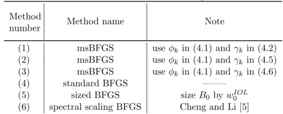
In this section, we show some numerical experiments. We used the 132 nonlin-ear unconstrained optimization problems in the CUTEr library [3]. We chose the test problems whose dimensions were between 499 and 1000. In Table 1, we give the methods examined in our experiments.

Table 1. Methods examined in our experiments Method

number Method name Note

(1) msBFGS use ϕk in (4.1) and γk in (4.2)

(2) msBFGS use ϕk in (4.1) and γk in (4.5)

(3) msBFGS use ϕk in (4.1) and γk in (4.6)

(4) standard BFGS ——–

(5) sized BFGS size B0 by wIOL0

(6) spectral scaling BFGS Cheng and Li [5]

In order to compare the proposed method with some existing BFGS type methods, we tested the standard BFGS, sized BFGS method, spectral scaling BFGS method and the msBFGS method based on (4.1), (4.2), (4.5) and (4.6). We number from (1) to (6) in Table 1. we tested the sized BFGS method (Method (5)) in which we sized B0 only at the first iteration by the inverse

Oren - Luenberger parameter ω₀IOL = y0B0−1y0

yT

0s0 . The spectral scaling BFGS

method (Method (6)) corresponds to Method (1) with ϕk = 0 and t = 0,

which is the Cheng - Li method.

All codes were written in C and run on a PC with 3.40 GHz CPU processor, 2.0GB RAM memory, and Linux operating system. We show the numerical results in Figures 1-5. In Figures 1-3, we stopped the iteration if the inequality

was satisfied, or if CPU time exceeded 600 seconds, and in Figures 4 and 5, we stopped the iteration if the inequality

∥gk∥∞≤ 10−8

was satisfied or if CPU time exceeded 600 seconds. For all examined methods, we chose the initial matrix B0 = I. For each method, to get the search

direction dk, we did not solve the linear system of equations Bkdk = −gk.

Instead we used the inverse updating formula as follows Hk+1 = Hk− HkyˆksT_k + sk(Hkyˆk)T ˆ yT_ksk + ( 1 γk +yˆ T kHkyˆk ˆ yT_ksk ) sksT_k ˆ yT_ksk .

In the line search, the step size αk was obtained so as to satisfy the Wolfe

conditions:

f (xk+ αkdk)≤ f(xk) + σ1αkgkTdk, g(xk+ αkdk)Tdk≥ σ2gTkdk,

where we chose σ1= 10−3 and σ2= 0.5.

We adopt the performance profiles by Dolan and Mor´e [8] to compare the performance of the methods based on the CPU time. We introduce the per-formance profile by Dolan and Mor´e. We assume that we are concerned with the set of solvers S, which has ns solvers, and the test set P, which has np

problems. For each problem p and solver s, let us define

tp,s= computing time required to solve problem p by solver s,

rp,s= tp,s min{tp,s: s∈ S} and ρs(ν) = 1 np |{p ∈ P : r p,s≤ ν}| .

The function ρs(ν) is the probability for solver s∈ S that a performance ratio rp,sis within a factor ν ∈ R of the best performance ratio. In Figures 1, 2 and

3, the function ρs(ν) distributes the curve, and the top curve is the method

which solved the most problems in a result that is within a factor ν of the best result.

Table 2. The parameter in a preliminary experiment Method number Values of parameters

(1) t∈ {0, 0.25, 0.5, 0.75, 1}, δk∈ [0, 10]

(2) l∈ {10−2, 10−1, 1, 10}, m, ¯M ∈ [10−7, 107], δk∈ [0, 10]

(3) t∈ {0, 0.25, 0.5, 0.75, 1}, ξ ∈ [10−2, 102_{], δ}

k∈ [0, 10]

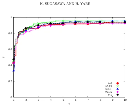
As a preliminary experiment, we chose the value of parameter for Method (1), (2), (3) in Table 2. In Figure 1, we examine Method (1) in which we always choose t = 1 and vary the value of δk. Figure 1 implies that Method

(1) with t = 1 has the tendency that the choice of the small value for δk

performs well. In our experiments, Methods (1), (2) and (3) have the similar tendency. However, the influence of δk is different a little for each method. As

shown in Figure 1, in some methods, by letting δk be a small positive value,

the performance becomes rather better than the case δk = 0. Meanwhile, in

some methods, even if we let δk be a small positive value, the performance

dose not. In Figure 2, we examine Method (1) in which we always choose δk= 10−5 and vary the value of t. Figure 2 shows that the parameter t hardly

affects the performance of Method (1). Moreover, in Method (3), we also find that the parameter t does not have big influence on computational efficiency.

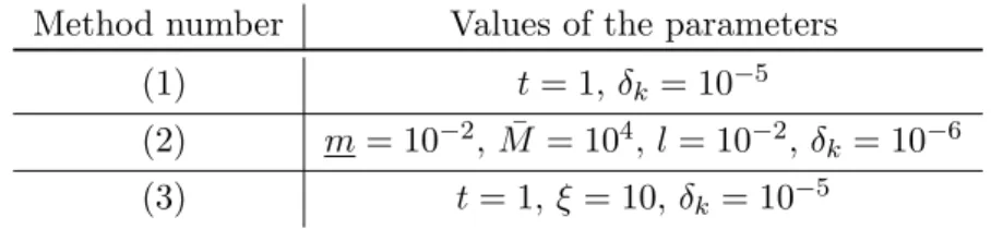
Table 3. The parameter values which give good numerical results Method number Values of the parameters

(1) t = 1, δk= 10−5

(2) m = 10−2, ¯M = 104, l = 10−2, δk= 10−6

(3) t = 1, ξ = 10, δk= 10−5

Next, we choose t = 1 and compare Methods (1)-(6). For this comparison, we first changed the parameter values in the range of Table 2 except t (however, the case δk = 0 is removed), and investigated which parameter values gave

good numerical results for every method. We show such values in Table 3. In Figure 3, we compare numerical performance of Methods (1)-(6) with the parameter values in Table 3. Figure 3 implies that Method (2) is the best solution, Method (3) is the second and Method (1) is the third. Hence, the msBFGS method with a suitable choice of the parameter values is superior to the standard BFGS method from the viewpoint of the CPU time. In particular, we observe that reducing the trace of Bk by Method (2) is efficient. However,

BFGS method even if we suitably chose m, ¯M and δk. Thus, it is preferable

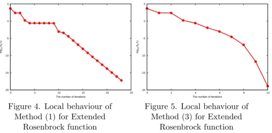
to select a small value for l. Furthermore, the results of Methods (1) and (3) imply that switching the scaling factor by (4.6) is efficient owing to the superliner convergence property of Method (3). In order to investigate the local behavior of Methods (1) and (3) with the parameter values in Table 3, in Figures 4 and 5, we compare the numerical results for solving the Extended Rosenbrock function (the problem 21 in [10]). These figures present the values of log₁₀|fk−f∗|, where f∗ denotes the optimal value. We can find that Method

(3) converges superlinearly for the Extended Rosenbrock function, but Method (1) dose not.

From the above observations, by choosing the parameter values suitably, our method performs effectively on the CPU time. Though we show the results only for the case t = 1 in Figure 3, we obtain similar results to Figure 3 for the other cases t (∈ {0, 0.25, 0.5, 0.75}), by selecting the parameter values suitably.

0 0.2 0.4 0.6 0.8 1 1 2 3 4 5 6 7 8 9 10 ρ τ δk=0 δk=10 -5 δk=10 -3 δk=10 -1 δk=1 δk=10

0 0.2 0.4 0.6 0.8 1 1 2 3 4 5 6 7 8 9 10 ρ τ t=0 t=0.25 t=0.5 t=0.75 t=1

 Figure 2. The case of choosing δk= 10−5 and varying t in Method (1)

0 0.2 0.4 0.6 0.8 1 1 2 3 4 5 6 7 8 9 10 ρ τ (1) (2) (3) (4) (5) (6)

Figure 3. The comparison between Methods (1)-(6) (use the parameter values in Table 3)

-20 -15 -10 -5 0 5 0 5 10 15 20 25 log 10 |fk -f* |

The number of iterations

Figure 4. Local behaviour of Method (1) for Extended

Rosenbrock function -20 -15 -10 -5 0 5 0 2 4 6 8 10 log 10 |fk -f* |

The number of iterations

Figure 5. Local behaviour of Method (3) for Extended

Rosenbrock function

§6. Conclusion

In this paper, we have proposed a modified scaling BFGS method (msBFGS) for unconstrained minimization, and proved the global and superliner con-vergence of our method. In addition, we have applied concrete parameters (scaling factors) to the msBFGS method, proved its convergence properties and done the numerical experiments. The numerical results show that our methods perform better in general than the standard BFGS method. As fur-ther works, we would apply a scaling factor to ofur-ther updating formulas.

Acknowledgments. The authors would like to thank the referee for valuable

comments. The second author is supported in part by the Grant-in-Aid for Scientific Research (C) 25330030 of Japan Society for the Promotion of Science.

References

[1] M. Al-Baali, Global and superlinear convergence of a restricted class of self-scaling methods with inexact line searches, for convex functions, Computational

Optimization and Applications 9 (1998), 191-203.

[2] M. Al-Baali, Numerical experience with a class of self-scaling quasi-Newton al-gorithms, Journal of Optimization Theory and Applications 96 (1998), 533-553. [3] I. Bongartz, A.R. Conn, N.I.M Gould and P.L. Toint, CUTE: Constrained and unconstrained testing environment, ACM Transactions on Mathematical

Soft-ware 21 (1995), 123-160.

[4] R.H. Byrd and J. Nocedal, A tool for the analysis of quasi-Newton methods with application to unconstrained minimization, SIAM Journal on Numerical

[5] W.Y. Cheng and D.H. Li, Spectral scaling BFGS method, Journal of

Optimiza-tion Theory and ApplicaOptimiza-tions 146 (2010), 305-319.

[6] J.E. Dennis, Jr. and J.J. Mor´e, A characterization of superlinear convergence

and its application to quasi-Newton methods, Mathematics of Computation 28 (1974), 549-560.

[7] J.E. Dennis, Jr. and J.J. Mor´e, Quasi-Newton methods, motivation and theory,

SIAM Review 19 (1977), 46-89.

[8] E.D. Dolan and J.J. Mor´e, Benchmarking optimization software with

perfor-mance profiles, Mathematical Programming 91 (2002), 201-213.

[9] D.H. Li and M. Fukushima, A modified BFGS method and its global convergence in nonconvex minimization, Journal of Computational and Applied Mathematics

129 (2001), 15-35.

[10] J.J. Mor´e, B.S. Garbow and K.E. Hillstrom, Testing unconstrained optimization

software, ACM Transactions on Mathematical Software 7 (1981), 17-41.

[11] J. Nocedal and Y. Yuan, Analysis of a self-scaling quasi-Newton method,

Math-ematical Programming 61 (1993), 19-37.

[12] J. Nocedal and S.J. Wright, Numerical Optimization, 2nd edn., Springer Series in Operations Research, Springer, New York, 2006.

[13] S.S. Oren, Self-scaling variable metric (SSVM) algorithms, Part II: Implementa-tion and experiments, Management Science 20 (1974), 863-874.

[14] S.S. Oren and D.G. Luenberger, Self-scaling variable metric (SSVM) algorithms, Part I: Criteria and sufficient conditions for scaling a class of algorithms,

Man-agement Science 20 (1974), 845-862.

[15] M.J.D. Powell, Updating conjugate directions by the BFGS formula,

Mathemat-ical Programming 38 (1987), 29-46.

[16] H. Yabe, H.J. Mart´ınez and R.A. Tapia, On sizing and shifting the BFGS update within the sized-Broyden family of secant updates, SIAM Journal on

Optimiza-tion 15 (2004), 139-160.

[17] Y. Yuan, A modified BFGS algorithm for unconstrained optimization, IMA

Jour-nal of Numerical AJour-nalysis 11 (1991), 325-332.

Kiyohisa Sugasawa

Sendai Signalling Communication Technical Center, East Japan Railway Company 31-2 Higashi6bancho, Miyagino-ku, Sendai-shi, Miyagi 983-0853, Japan

E-mail : [email protected]

Hiroshi Yabe

Department of Mathematical information Science, Tokyo University of Science 1-3 Kagurazaka, Shinjuku-ku, Tokyo 162-8601, Japan